
19.1: Engineering and Science Languages
- Page ID
- 43118
Here we present some of the programming languages that are useful for engineering and science.
IDL
This is a science language primarily used by astronomers but can be used by engineers. It's design centers around image processing for science. With that in mind it has a matrix-style ability similar to Octave. We will introduce IDL here and give an example using one of the routines from NASA/GSFC.
IDL is primarily used at NASA/GSFC, NIST, and NIH. At NASA/GSFC, it mostly supplanted the previous scientific image processing language, IRAF, though there is still some people who still used IRAF instead of IDL. The language has a host of routines available which we will detail later. GDL is a open source programming language that is highly compatible with IDL and can be used as an alternative to IDL especially in academic areas where financing is an issue. While GDL is not as powerful as IDL it offers a number of features that IDL offers in a similar syntax very much like Octave is to MATLAB.
- IDL/GDL is matrix-based (which is how image processing is done) like Octave/MATLAB/Scilab
- PV-WAVE comes from IDL but has evolved from it but it still has the looks of IDL
- In comparison IDL and GDL are almost alike like Octave and MATLAB, PV-WAVE diverges enough to be distinct but very similar like Scilab does
Routines for science and engineering
For IDL to be used effectively you would need routines that have been developed previously. This is no different then Python or Octave except that IDL does not have one general place to get routines but many web sites. Here is an incomplete list.
- David Fanning's IDL site - this is one of the top IDL web sites, however it is not as active as it once one
- https://people.ast.cam.ac.uk/~vasily/idl.htm - general site that offers some information and links to other web sites
- https://michaelgalloy.com/wp-content/uploads/2006/10/operators.pdf - Useful pdf of the operators in IDL
- NIH
- Unfortunately most of NIH software is protected and needs a password unlike NASA/GSFC which is more open
- NIH uses IDL but also uses MATLAB and Mathematica
- NIST
- DAVE is an analysis environment developed on top of IDL
- NASA and NASA-related sites
- The IDL Astronomy User's Library (also know as IDLASTRO - can download routines from github - Wayne Landsman's area)
- DanDL - Science and Astronomy
- WMAP software - actually a mixture of Fortran and IDL
- RVLIN - exoplanet software
- NICMOSlook - this is pretty old IDL code and program, but it can be used as an example (and if you want to analyze NICMOS data)
- "SGP-IDL" program - the IDL program is on the bottom of the page (MATLAB programs are on the top)
- JHU-APL library page - useful library of IDL routines that is heavily used by NASA
And now an example for IDL, but first we need to introduce a transform, Radon Transform. The Radon transform is an integrating transform that is typically used in tomography (imaging by sections) but is also used in barcode scanners, seismology, and in removing certain types of noise in imaging which includes astronomy. This transform is related to the Fourier transform which as you know is one of the most important transforms in engineering and science (remember FFT). In simple terms it reconstructs an image from scattered data pieces of a volume (hence tomography). Similar transforms include the Minkowski-Funk transform (Funk), the Hough transform (which is good for line detection unless your data is noisy with speckles then you should use the Radon transform), and the Penrose transform (which is just a complex version of the Radon transform).
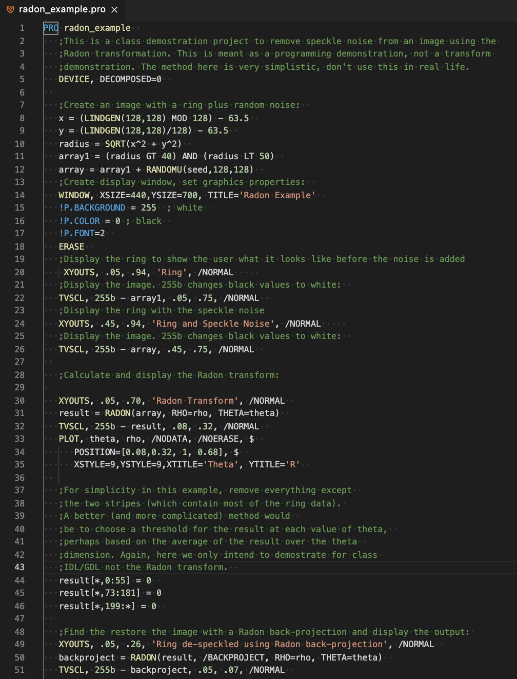
All this might sound a bit technical at this point but as time goes on and you learn more you will be amazed how this becomes a sort of second nature. Below is a GDL script that utilizes the Radon transform from IDLASTRO. But before that let us review what we are going to do.
Example
- Generate a ring with speckle noise - this will represent our noisy data
- Take the Radon transform (RADON) of the data and display that (just to show you)
- Remove everything in the transform except the stripes (this is not the best approach - better approaches would obscure the message though)
- Using the Randon back-projection reconstruct the image de-speckled
- This is run in gdl so you can try it to if you get the open source program!
 |
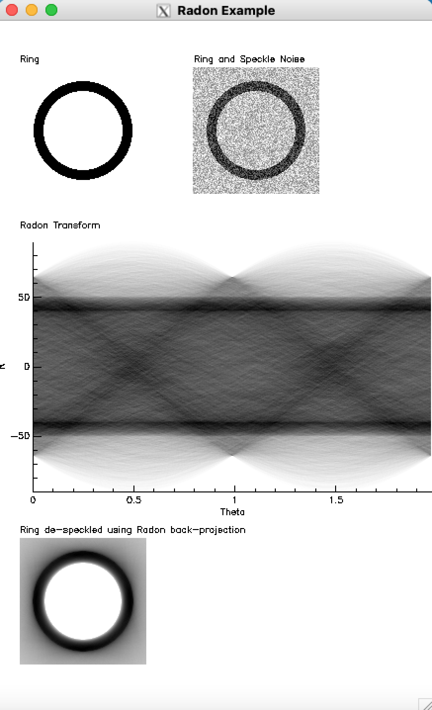 |
| GDL programming demonstrating some image processing as might be found in science/engineering. Examine this program thoroughly and try to understand each command (use web sources to help if you wish - that is what would be done in the "real world"). | This is the result of the GDL program on the speckled noise test algorithm. As you can see the speckle noise is removed, however the background seems to have become noisy on the edges (though not the center). Improvement of this process can be used to de-speckle noises in astronomy images or medical images without the noise that is still in the result here. |
Python
Python is technically not a scientific programming language, however, through packages that can be obtained at the Python Package Index (pypi not to be confused with pipi which is another type of Python) you can use it as a scientific language. Octave/MATLAB/Scilab also have packages for additional scientific abilities though they have a lot more built-in then Python. These packages are a must if you want to do scientific/engineering work with Python.
Packages
Python has "modules" which contain pre-defined functions that our collected together to make package. These packages are essential for useful work with Python. For Python and in particular for science you would need the following packages at a minimum:
- Matplotlib - Python plotting package that you really need to do any plotting
- NumPy - Python package for computation especially with matrices
- SciPy - Python's scientific library (note SciPy has an "ecosystem" and has it's own web site: SciPy.org)
- Check out the pypi and scipy for more packages
Examples
- This is simple examples of some of NumPy's abilities.
- A simple example using NumPy and Matplotlib.
- A simple example using SciPy. Here we have our data, a linear interpolation, and fit using a cubic spline. This complements the previous disussions by showing an example of fitting to a curve. The spline is very close to the data (which is a function that can be graphed if you want to see what it should look like...your assignment).
Octave
Octave, MATLAB, and Scilab are science languages primarily used by engineers but can be used by scientists. This languages are designed to easily do matrix mathematics which is very important in engineering. Octave and MATLAB are almost completely compatible whereas Scilab is mostly compatible but does have some differences. MATLAB as a paid project is more functionality then either Octave or Scilab, but Octave or Scilab is excellent for those on a budget.
While a lot of science features are included in the core program for these languages so there is less need to go to packages (or toolboxes as MATLAB and Scilab calls them). However for some special functions these programs do have packages.
Octave Forge Packages
Octave packages can be found in many locations, but the best list of packages is at Octave Forge. For MATLAB and Scilab it is best just to go to the website and search for toolboxes. Note you have to pay for the toolboxes as well as the product for MATLAB. Scilab like Octave is open source so that is not an issue with that software.
Key Packages:
- octave-optim — non-linear optimization tools, but in particular wpolyfit which is used in laboratory herein
- octave-control — control system design functions; transfer function creation; bode plot
- octave-signals — signal generation and signal analysis tools includes IIR filter design routines; this is an absolute must
- octave-splines — splines are an extremely important tool; this package is a must
- octave-linear-algebra — linear algebra is need for control systems
- octave-gsl — binds octave to functions in the gnu science library (see C example below)
- octave-mechanics — functions useful for mechanics included in this is some molecular dynamics routines (which is not exactly mechanics)
- octave-quaternion — quaternion procedures that were found in mechanics originally but have since split off and expanded
- octave-symbolic — this gives octave the ability to manipulate symbols like MATLAB using Python's SymPy
- This is not a must; this is just if you want to do symbolic mathematics
- The authors believe that maxima would be better for this though; use wxMaxima/maxima instead
- wxMaxima/maxima is like Mathematica however it is older then Mathematica
- maxima's origins are from the 1960s (Macsyma:MIT:Lisp-based)
- Interestingly because Macsyma required computers that were more expensive than the general user could afford a competitor to it was developed in the 1980s called Maple (University of Waterloo:B programming language)
- As you might expect B was before the C programming language
- Now however maxima can be run on laptops; while Maple still exists its original motivation is no longer relevant
Example
Example of octave has already been done extensively throughout this course/book. See the previous examples. May add one later here, but not for now.
Fortran (and C and C++)
Fortran is a programming language designed for science but it depends on libraries extensively to provide the best science functions (this is true of C and C++ as well). These libraries are like the packages of the interpretive science languages like Octave/MATLAB/Scilab or IDL/GDL. Frequently, the compiled libraries of Fortran and C/C++ are the basis of the packages in the interpretive science languages.
If these libraries are the source of most packages out there why not just go straight to the source? Because for most people these libraries are more complicated (less user friendly) and take extra effort to learn (which is valuable however). Some advantages of the libraries is that by editing and compiling these routines you can, with learned skill, speed up your programs and even add special cases that are not generally represented in routines that you might need. For the interpretive science languages you might be stuck with what you get. Still most people don't have major special cases and the ease of use makes the interpretive science languages' packages attractive.
This is where we would go back to numerical methods because most of the libraries/packages are based off the concepts in numerical methods.
Numerical Methods aspect of libraries
Numerical methods boil down to methods of approximating physical problems that are intractable using analytic techniques. Key ideas:
- Physical problems are represented by mathematical equations
- Parachute person was an simplistic example of this
- For real world problems you are liking to have multiple equations and following the systems example in the fundamental portion of this course we can see that almost any real world problem can be represented by this
- Or to put it another way n unknowns and n equations
- In order to solve n unknowns and n equations we would resort to matrices (hence the popularity of Octave/MATLAB)
- In real world problems this n equations are actually differential equations, but the same matrices principles apply
- A number of approximation techniques are available for the same physical expressing and are used depending on the conditions
- This techniques do have methods of assigning error
- Assigning error can be a difficult task
- This is an area where you might want to modify a program to fit the error analysis you believe is appropriate (when you are an expert!)
- Any of the routines found in the packages can be designed and written from scratch, however, these have existed and been regularly corrected for a long time so unless you truly have some evidence that there is a problem, best just use the libraries
Sample of numerical methods packages
Most of the numerical methods packages commonly used can be found on the NETLIB web site (either on the site or a link to another site - usually NIST). This libraries are written in Fortran, C, and C++. This does not mean that only Fortran libraries can be read by Fortran. C can read Fortran and C++ libraries, Fortran can read C and C++ libraries, and C++ can read Fortran and C libraries. You may need to take some extra care doing this, but most modern compilers make this rather easy.
Originally most of these libraries were written in Fortran but now most have been convert to C (and C++). If you want to investigate this programs it is probably better to look at the descriptive list at http://www.netlib.org/master/expanded_liblist.html.
Key libraries:
- EISPACK — Eigenvalue and eigenvector library (Fortran, note LAPACK has most of these routines now)
- LINPACK — Linear algebra pack (Fortran, note LAPACK has most of these routines now, with improvements)
- LAPACK — Modern linear algebra pack
- MINPACK — Non-linear problems
- NAPACK — Numerical linear algebra and optimization pack (Fortran)
- ODEPACK — Differential equations package
- QUADPACK — Integration package - generally incorporated into interpretive programs now
- FFTPACK — FFTs, of course
- SLAP — Sparse Linear Algebra Package
- BLAS — Basic Linear Algebra subprograms
GNU has rewritten a lot of these packages (in C and C++; but can be used in any language given binding abilities of modern languages) and more to form the GNU scientific library (gsl). If you look at the reference manual you will see references to NETLIB. The GNU scientific library is extensive.
Examples
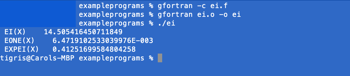
- Fortran using a routine from NETLIB
 |
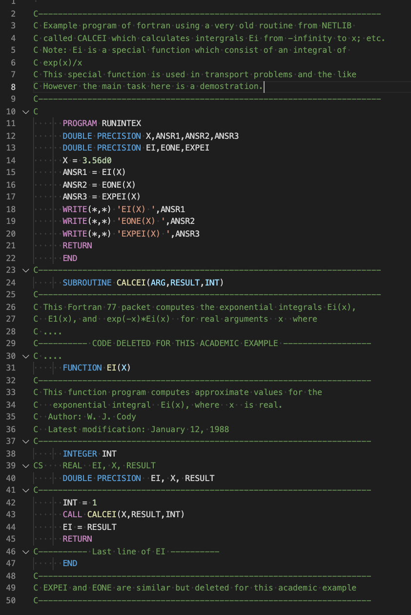 |
| This is a Fortran example program using a NETLIB subroutine to do some engineering/science calculation. Note the compiling and linking of Fortran to produce the program ei, before we run it (./ei). We did not use a library here, but if we did we would need either a static library (*.a) or a dynamic library (*.so). Fortran includes a lot of science functions by default so the need to link in a library may not be needed in most instances. These default functions are referred to as intrinsic procedures. | A little program was written on top of this NETLIB subroutine to demonstrate how you might used it. Bits of the code from NETLIB subroutine are displayed for context, but you should access the actual code at NETLIB to get a full measure of it's scope (look for ei in specfun). Note if you do use this routine there are comments (CS, CD) that need to be uncommented depending if you are using single or double precision (here we used double precision so you do not see the CD comment marks as they were deleted) |
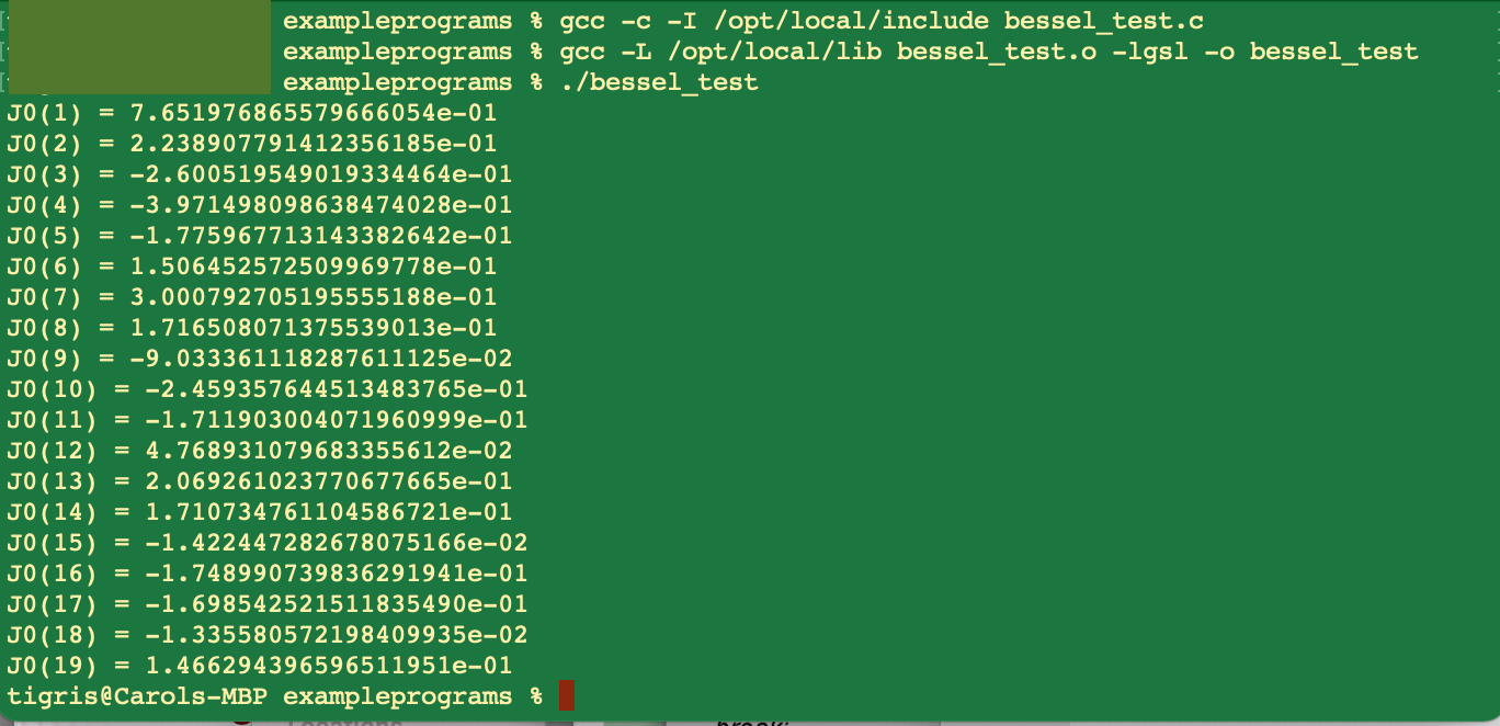
- C using gnu scientific library (gsl)
 |
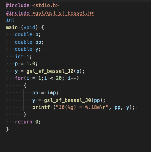 |
| This is the run on the C program on the left. Before that is the compiling of the program and the linking of the program. The first line is compiling of the program requires the author to tell the compiler where the gsl include file was (-I /opt/local/include). The second line is the linking of the program. The gsl library was linked by option -lgsl and again the author had to tell the compiler where the gsl library was (-L /opt/local/lib). Note the compiling and linking can be combined, but the author likes to check his syntax first before he links (otherwise it is harder to distinguish between syntax errors and linking errors). | This is a simple C program to calculate the Bessel function at different values. C is very close to C++ so only minor modifications need to be made if you want to use C++. Note the include files are for the gnu scientific library (gsl/gsl_sf_bessel.h) and is the way we get the Bessel function (gsl_sf_bessel_J0). We still need to connect to this include file and function through the compile. See the example to the left. |