28.4: Switching Polarisation

In an electric field, E, a polarised material lowers its (volume-normalized) free energy by –P.E, (where P is the polarisation). Any dipole moments which lie parallel to the electric field are lowered in free energy, while moments that lie perpendicular to the field are higher in free energy and moments that lie anti-parallel are even higher in free energy, (+P.E).

This introduces a driving force to minimise the free energy, such that all dipole moments align with the electric field.

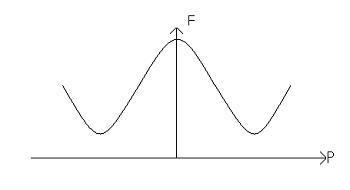
Let us start by considering how dipole moments may align in zero applied field:

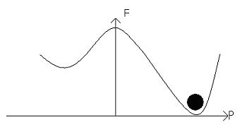
These two moments are stable, because they sit in potential energy wells. The potential barrier between them can be represented on a free energy diagram:

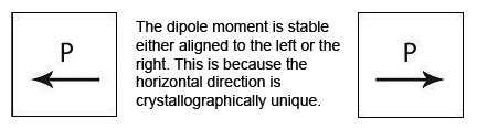
This material is considered to be homogenous. If the polarisation points left then we have:

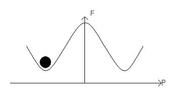
The electric field alters the free energy profile, resulting in a ‘tilting’ of the potential well:

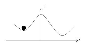
An increase in the electric field will result in a greater tilt, and lead to the dipole moments switching, leading to:

Next we must look at the more realistic scenario in which domains form.

Consider a material which is fully polarised, so that all of the dipole moments are aligned in the same direction. Then apply a reversed electric field over it. New domains with a reversed polarisation nucleate inhomogenously. This requires a certain amount of time, in the same manner as any nucleation process. When the fluctuating nuclei reach a certain critical radius, they grow outwards, forming needle-like structures. When they reach the other side of the ferroelectric, they begin to grow outwards.

This shows the origin of the hysteresis loop. The removal of the field will leave some polarisation behind, and only when the field is reversed does the polarisation start to lessen as new, oppositely poled domains form. They grow quickly however, giving a large change of polarisation for very little electric field. But to form an entirely reversed material, a large switching field is required. This is because of both defects in the crystal structure, in a manner similar to zener drag, and also to do with stray field energy. The polarisation of the material goes from a coupled pattern, with 180° boundaries, to a state in which many heads and tails are separated. This leads to the increase in stray field energy. Therefore, to attain this state, lots of energy has to be put in by a larger field.

Here we show a how a minor hysteresis loop fits into the major loop above.

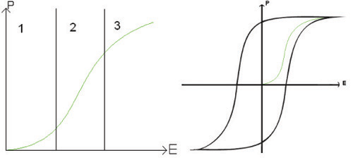
The part of curve shown fits into the major hysteresis curve.

There are three sections to this curve.
1) Reversible domain wall motion.
2) Linear growth of new domains.
3) New domains reaching the limit of their growth.