1.5: Limit Analysis

The concept of a lower bound has been introduced with reference to the work formula approach to analyse deformation. This approach generally results in an underestimate of the required load. Clearly, there also will be an “upper bound”, i.e. an overestimate of the load that needs to be applied to effect a given deformation. The two approaches together are called “limit analysis” since the actual loads required will lie between the lower and upper bounds. In practice, limit analysis is much easier to apply to a problem than the slip-line field approach and can be reasonably accurate. The upper bound is particularly useful for the study of metalworking processes in which it is essential to ensure sufficient forces are applied to cause the required deformation. In contrast, the lower bound is valuable in engineering where failure of a component must be avoided and hence an estimate of the minimum collapse load is needed.

The approach taken for estimating the upper bound is based on suggesting a likely deformation pattern, i.e. lines along which slip would be expected to occur for a given loading situation. Then the rate at which energy is dissipated by shear along these lines can be calculated and equated to the work done by an (unknown) external force. By refining the geometry of the deformation pattern, the minimum upper bound can be determined. Frictional forces can be accommodated in this approach. The approach utilises hodographs, which are self-consistent plots of velocity for different regions within a body being deformed; the different regions are assigned by considering how the overall body will deform for a particular deformation process and their relative velocities are estimated by assuming that the applied external force has unit velocity.

For both upper- and lower-bounds, one of the following two conditions has to be satisfied:

• geometrical compatibility between internal and external displacements or strains. This is usually concerned with kinetic conditions – velocities must be compatible to ensure no gain or loss of material at any point.
• stress equilibrium i.e. the internal stress fields must balance the externally applied stresses (forces).

The basis of limit analysis rests upon two theorems, which can be proved mathematically. In simple terms, these theorems are:

1. Lower Bound: any stress system in which the applied forces are just sufficient to cause yielding.
2. Upper Bound: Any velocity field that can operate is associated with an upper bound solution.

Example \(\PageIndex{1}\): Notched bar in tension

The plane strain condition is satisfied when breath, \(b » h\), the depth of the bar.

Lower-Bound:

Find a stress system, e.g. \( \sigma = 0\) in the length of the bar where there is the notch, \(\sigma = 2k\) elsewhere.

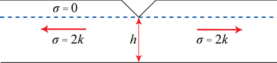
Therefore, for a breadth \( b \), \( P = 2khb = \text{load} = \text{stress} \times \text{area} \)

Upper-Bound:

Postulate a suitable simple deformation pattern.

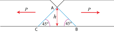
Assume yielding by slip on 45º shear planes with shear yield stress k. Let displacement along shear plane \( \mathrm{AB}=\delta x \).

Then internal work done = \( k .|A B| b \delta x=k \sqrt{2} b h \delta x\), where the force is \( k\left| {AB} \right|b \) acting on the shear plane AB.

Distance moved by the external load \(P=\delta x \cos 45^{\circ}=\frac{\delta x}{\sqrt{2}}\)

\[\Rightarrow P \frac{\delta x}{\sqrt{2}}=k \sqrt{2} b h \delta x \]

\[\Rightarrow P = 2kbh\]

So, here we obtain the same result for the upper bound and lower bound \( \Rightarrow P = 2kbh\) is the true failure load, the load required to cause plastic flow.

Example \(\PageIndex{2}\): Notched bar in plane bending

Lower-Bound:

The area immediately under the notch, above the neutral axis is in tension \( \sigma=2 k \). The area below the neutral axis is in compression \( \sigma=2 k \).

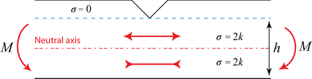
where:

\( h \) = thickness of slab beneath the notch.

\( 2 k . \frac{h}{2} \cdot b \) = magnitude of forces in tensile and compressive regions.
\( \frac{h}{2} \) = distance between the two.

Equating the couples,

\[ M=\left(2 k . \frac{h}{2} \cdot b\right) \frac{h}{2}=0.5 k h^{2} b \]

Upper-Bound:

Assume failure occurs by sliding around a ‘plastic hinge’ along a circular arc of length l and radius r.

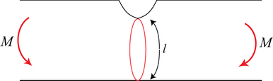
If the rotation is δθ, the internal work done \( =k . l b . r \delta \theta \) along one arc.

External work \( =M \delta \theta \) by one moment.

\[ \Rightarrow M=k l b r \]

where no assumptions have been made regarding l and r.

The upper bound theorem states that whatever values are taken for l and r will lead to an upper bound. Clearly we wish to find the lowest possible value.

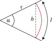
From the above geometry,

\[ l=r \alpha \]

and

\[ r=\frac{h}{2 \sin \alpha / 2} \]

\[\Rightarrow M=\frac{k h^{2} b}{4} \frac{\alpha}{\sin ^{2} \alpha / 2}\]

and so to find the lowest possible value of M, we minimize the function \( \dfrac{\alpha}{\sin ^{2} \alpha / 2} \)

Let

\[ Y=\frac{\alpha}{\sin ^{2} \alpha / 2} \nonumber \]

\[ \frac{\mathrm{d} Y}{\mathrm{d} \alpha}=\frac{1}{\sin ^{4} \alpha / 2}\left\{\sin ^{2} \frac{\alpha}{2}-2 \frac{\alpha}{2} \cos \frac{\alpha}{2} \sin \frac{\alpha}{2}\right\} \nonumber \]

\[ =0 \quad \text { when } \quad \sin \frac{\alpha}{2}=\alpha \cos \frac{\alpha}{2} \nonumber \]

\[ \Rightarrow \tan \frac{\alpha}{2}=\alpha \nonumber \]

\[ \Rightarrow M=\frac{k h^{2} b}{4} \cdot \frac{1}{\sin \alpha / 2 \cos \alpha / 2}=1 / 2 \frac{k h^{2} b}{\sin \alpha} \cong 0.69 k h^{2} b \nonumber \]

Taking the lower bound and the upper bound as limits, we therefore find

\[\Rightarrow 0.5 \leq \frac{M}{k h^{2} b} \leq 0.69 \nonumber \]

This forms a good example of constraining the value of the external force between lower bound and upper bound. It is also a good example of how to produce a lower limit on an upper bound calculation.

Hodographs I

A hodograph is a diagram showing the relative velocities of the various parts of a deformation process. To analyze a complicated deformation process with many shear planes, it is worth looking at the basic equation for the rate of energy dissipation in an upper bound situation in more detail.

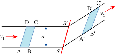
ABCD is distorted into A'B'C'D' by shear along \(\overrightarrow {SS`} \) at a velocity \( \underline{v_{s}} \) in the metal.

Suppose ABCD moves towards the shear plane SS' at a velocity \({v_1}\) and suppose that there is a pressure P acting on the area al (where l is the dimension out of the plane of the paper) helping to cause this movement.

Rate of performance of work externally \( = pal\left| \underline {v_1} \right|\)

Rate of performance of work internally \( = k\left| {SS`} \right|l\left| \underline{v_s} \right|\)

since the only internal work assumed to occur is that required to effect the shear deformation so that ABCD → A'B'C'D'.

Equating these,

\[ \Rightarrow p a\left|\underline{v_{1}}\right|=k\left|S S^{*}\right|\left|\underline{v_{s}}\|\right. \]

\[\Rightarrow p a=k\left|S S^{*}\right| \frac{\left|v_{s}\right|}{\left|v_{1}\right|} \]

Simple vector algebra relates v₁, v₂ and v_s as on the diagram below:

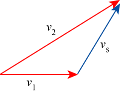
If in a deformation process there are n such shear planes of the type SS', then \( p a=k \sum_{n}\left|S S_{n}^{s}\right|\left|v_{s n}\right| \) setting \( \left|\underline{v_{1}}\right|=1.0\), i.e. unit velocity.

Rules for constructing a hodograph

The animation below illustrates the seven rules for constructing a hodograph, for the case of a constrained punch.

Note: This animation requires Adobe Flash Player 8 and later, which can be downloaded here.

An analysis of the geometry of the hodograph enables an upper bound for the applied force to be calculated.

Let \( Oq \) be a velocity vector of unit magnitude in the hodograph, i.e. \( ν_{Oq} = 1 \)
Due to the dead metal zone, Q and Q' move at the same velocity.
\( O \) is a stationary component of the system, anywhere in the surrounding perfectly rigid metal which has not yielded at all.
\( Oq \) and \( Oq' \) are in essence vectors defining the motion of particles in region Q'.
Or is velocity of a particle in region R.
q'r is a vector defining the shear velocity parallel to Q'R.
Os is velocity of a particle in region S.
rs is a vector defining the shear velocity parallel to RS.

Hence,

\[ v_{O r}=\frac{1}{\tan \theta}, v_{q^{\prime} r}=\frac{1}{\sin \theta} \text { and } v_{O s}=v_{r s}=\frac{1}{2 \sin \theta} \nonumber \]

\( \Rightarrow \) Using the rate of performance of work formula we have:

\[p\left( {\frac{b}{2}} \right) = k\left\{ {Q'R{v_{q'r}} + OR{v_{Or}} + RS{v_{rs}} + OS{v_{Os}}} \right\}\]

where Q'R is the length of the line dividing regions Q' and R, OR is the length of the line dividing regions O and R, RS is the length of the line dividing regions R and S and OS is the length of the line dividing regions O and S

\[p\left(\frac{b}{2}\right)=k b\left\{\frac{1}{2 \cos \theta} \cdot \frac{1}{\sin \theta}+1 \cdot \frac{1}{\tan \theta}+\frac{1}{2 \sin \theta} \cdot \frac{1}{2 \sin \theta}+\frac{1}{2 \cos \theta} \cdot \frac{1}{2 \sin \theta}\right\} \nonumber \]

\[ =k b\left\{\frac{1}{\sin \theta \cos \theta}+\frac{\cos \theta}{\sin \theta}\right\}=k b\left\{\frac{1+\cos ^{2} \theta}{\cos \theta \sin \theta}\right\} \nonumber \]

\[ \Rightarrow \frac{p}{2 k}=\frac{1+\cos ^{2} \theta}{\sin \theta \cos \theta}=f(\theta) \nonumber \]

\( \frac{d f}{d \theta}=0 \) and \(f \)is then a minimum when

\[ \cos 2 \theta=-\frac{1}{3} \Rightarrow \theta=54.74^{\circ} \text { when } \sin \theta=\frac{\sqrt{2}}{\sqrt{3}} \text { and } \cos \theta=\frac{1}{\sqrt{3}} \nonumber \]

\( \Rightarrow \) minimum \(\dfrac{p}{2k}\)\( = 2\sqrt 2 = 2.83\) from this upper bound analysis.

When indenting using a sliding (frictionless) punch, we can postulate a different deformation pattern without the dead metal zone. The system also has a plane of symmetry and a hodograph can be constructed as follows:

Note: This animation requires Adobe Flash Player 8 and later, which can be downloaded here.

As before, \( O_q = 1.0 \)

Material in R travels in direction shown with velocity \( Or = \frac{1}{\sin \theta } \)

\[ |O r|=|r s|=\frac{1}{\sin \theta}=|s t|=|O t| \nonumber \]

\[ \left| {Os} \right| = \frac{2\cos \theta }{\sin \theta } \nonumber \]

\[ \left| {qr} \right| = \frac{1}{\tan \theta }= \frac{\cos \theta }{\sin \theta } \nonumber \]

Lengths in drawing of indent: \(QR = SO = \dfrac{b}{2}\)

\[ OR = RS = ST = OT = \dfrac{b}{4\cos \theta} \]

We therefore have:

\( \dfrac{pb}{2}\) = \(k\left\{ OR{v_{Or} + RS{v_{rs}} + OS{v_{Os}} + ST{v_{st}} + TO{v_{tO}}} \right\} \)

\[ =k b\left\{\frac{1}{4 \cos \theta} \cdot \frac{1}{\sin \theta}+\frac{1}{4 \cos \theta} \cdot \frac{1}{\sin \theta}+\frac{1}{2} \cdot \frac{2 \cos \theta}{\sin \theta}+\frac{1}{4 \cos \theta} \cdot \frac{1}{\sin \theta}+\frac{1}{4 \cos \theta} \cdot \frac{1}{\sin \theta}\right\} \nonumber \]

\[ =k b\left\{\frac{1}{\sin \theta \cos \theta}+\frac{\cos \theta}{\sin \theta}\right\} \nonumber \]

\( \Rightarrow \dfrac{P}{2 k}=\left\{\dfrac{1+\cos ^{2} \theta}{\sin \theta \cos \theta}\right\} \) as before for the case of the constrained punch.

This analysis has assumed that no friction occurs at the punch face to cause particles in R to move parallel to OR. If there is friction, we can take it to be sticking friction, so that there is a shear stress k acting and slippage velocity \( = {v_{qr}}\)

\( \Rightarrow \) in this case \(\frac{P}{2k}\) = \(\left\{ \frac{2 + 3{\cos }^2 \theta }{2\sin \theta \cos \theta } \right\}\)

\( \Rightarrow \) of the three possible upper bound solutions, the 'best' answer is \(\frac{P}{2k}\) = \(2\sqrt 2 = 2.83\)

This is a 10% overestimate of the true value of \(\dfrac{P}{2k}\) found from slip-line field theory.

Hodographs II

Extrusion is an important working process. A simple form of extrusion used for non-ferrous metals involves a smooth square die.

We define extrusion ratio, R = ratio of areas.

\( R=\frac{A_{0}}{A_{1}}=\frac{H}{h} \) for plane strain (R > 1), e.g. R = 4 = 75% reduction in area.

For a square die with sliding on the die face in plane strain, the hodograph can be constructed as follows:

Note: This animation requires Adobe Flash Player 8 and later, which can be downloaded here.

Click here for a full mathematical analysis of this hodograph.

An alternative approach to an extrusion hodograph assumes there is a 'dead metal' zone.

Note: This animation requires Adobe Flash Player 8 and later, which can be downloaded here.

Then

\[ p \frac{H}{2}=k\left\{P Q v_{P Q}+D Q v_{d q}+Q R v_{q r}\right\} \]

After similar algebra to the previous example, we obtain

\[ \frac{p}{2 k}= \frac{1}{2(\sin \varphi-\cos \varphi)} \left\{\frac{R+1}{\sin \varphi}-2(R-1) \cos \varphi\right \} \]

Minimising \( \cot \varphi=1-\frac{2}{\sqrt{R+1}} \)

After more algebra, it is found that

\[ \frac{p_{\min }}{2 k}=2(\sqrt{R+1}-1) \]

Note that for low R (< 4) this value is less than that for sliding on the die face, even if the die face is frictionless.

⇒ For R < 4 this is a better upper bound solution for extrusion problems.

Click here for a full mathematical analysis of this hodograph.