Engineering LibreTexts

1.4: Work Formula Method

  • Page ID
    7782
  • \( \newcommand{\vecs}[1]{\overset { \scriptstyle \rightharpoonup} {\mathbf{#1}} } \)

    \( \newcommand{\vecd}[1]{\overset{-\!-\!\rightharpoonup}{\vphantom{a}\smash {#1}}} \)

    \( \newcommand{\id}{\mathrm{id}}\) \( \newcommand{\Span}{\mathrm{span}}\)

    ( \newcommand{\kernel}{\mathrm{null}\,}\) \( \newcommand{\range}{\mathrm{range}\,}\)

    \( \newcommand{\RealPart}{\mathrm{Re}}\) \( \newcommand{\ImaginaryPart}{\mathrm{Im}}\)

    \( \newcommand{\Argument}{\mathrm{Arg}}\) \( \newcommand{\norm}[1]{\| #1 \|}\)

    \( \newcommand{\inner}[2]{\langle #1, #2 \rangle}\)

    \( \newcommand{\Span}{\mathrm{span}}\)

    \( \newcommand{\id}{\mathrm{id}}\)

    \( \newcommand{\Span}{\mathrm{span}}\)

    \( \newcommand{\kernel}{\mathrm{null}\,}\)

    \( \newcommand{\range}{\mathrm{range}\,}\)

    \( \newcommand{\RealPart}{\mathrm{Re}}\)

    \( \newcommand{\ImaginaryPart}{\mathrm{Im}}\)

    \( \newcommand{\Argument}{\mathrm{Arg}}\)

    \( \newcommand{\norm}[1]{\| #1 \|}\)

    \( \newcommand{\inner}[2]{\langle #1, #2 \rangle}\)

    \( \newcommand{\Span}{\mathrm{span}}\) \( \newcommand{\AA}{\unicode[.8,0]{x212B}}\)

    \( \newcommand{\vectorA}[1]{\vec{#1}}      % arrow\)

    \( \newcommand{\vectorAt}[1]{\vec{\text{#1}}}      % arrow\)

    \( \newcommand{\vectorB}[1]{\overset { \scriptstyle \rightharpoonup} {\mathbf{#1}} } \)

    \( \newcommand{\vectorC}[1]{\textbf{#1}} \)

    \( \newcommand{\vectorD}[1]{\overrightarrow{#1}} \)

    \( \newcommand{\vectorDt}[1]{\overrightarrow{\text{#1}}} \)

    \( \newcommand{\vectE}[1]{\overset{-\!-\!\rightharpoonup}{\vphantom{a}\smash{\mathbf {#1}}}} \)

    \( \newcommand{\vecs}[1]{\overset { \scriptstyle \rightharpoonup} {\mathbf{#1}} } \)

    \( \newcommand{\vecd}[1]{\overset{-\!-\!\rightharpoonup}{\vphantom{a}\smash {#1}}} \)

    \(\newcommand{\avec}{\mathbf a}\) \(\newcommand{\bvec}{\mathbf b}\) \(\newcommand{\cvec}{\mathbf c}\) \(\newcommand{\dvec}{\mathbf d}\) \(\newcommand{\dtil}{\widetilde{\mathbf d}}\) \(\newcommand{\evec}{\mathbf e}\) \(\newcommand{\fvec}{\mathbf f}\) \(\newcommand{\nvec}{\mathbf n}\) \(\newcommand{\pvec}{\mathbf p}\) \(\newcommand{\qvec}{\mathbf q}\) \(\newcommand{\svec}{\mathbf s}\) \(\newcommand{\tvec}{\mathbf t}\) \(\newcommand{\uvec}{\mathbf u}\) \(\newcommand{\vvec}{\mathbf v}\) \(\newcommand{\wvec}{\mathbf w}\) \(\newcommand{\xvec}{\mathbf x}\) \(\newcommand{\yvec}{\mathbf y}\) \(\newcommand{\zvec}{\mathbf z}\) \(\newcommand{\rvec}{\mathbf r}\) \(\newcommand{\mvec}{\mathbf m}\) \(\newcommand{\zerovec}{\mathbf 0}\) \(\newcommand{\onevec}{\mathbf 1}\) \(\newcommand{\real}{\mathbb R}\) \(\newcommand{\twovec}[2]{\left[\begin{array}{r}#1 \\ #2 \end{array}\right]}\) \(\newcommand{\ctwovec}[2]{\left[\begin{array}{c}#1 \\ #2 \end{array}\right]}\) \(\newcommand{\threevec}[3]{\left[\begin{array}{r}#1 \\ #2 \\ #3 \end{array}\right]}\) \(\newcommand{\cthreevec}[3]{\left[\begin{array}{c}#1 \\ #2 \\ #3 \end{array}\right]}\) \(\newcommand{\fourvec}[4]{\left[\begin{array}{r}#1 \\ #2 \\ #3 \\ #4 \end{array}\right]}\) \(\newcommand{\cfourvec}[4]{\left[\begin{array}{c}#1 \\ #2 \\ #3 \\ #4 \end{array}\right]}\) \(\newcommand{\fivevec}[5]{\left[\begin{array}{r}#1 \\ #2 \\ #3 \\ #4 \\ #5 \\ \end{array}\right]}\) \(\newcommand{\cfivevec}[5]{\left[\begin{array}{c}#1 \\ #2 \\ #3 \\ #4 \\ #5 \\ \end{array}\right]}\) \(\newcommand{\mattwo}[4]{\left[\begin{array}{rr}#1 \amp #2 \\ #3 \amp #4 \\ \end{array}\right]}\) \(\newcommand{\laspan}[1]{\text{Span}\{#1\}}\) \(\newcommand{\bcal}{\cal B}\) \(\newcommand{\ccal}{\cal C}\) \(\newcommand{\scal}{\cal S}\) \(\newcommand{\wcal}{\cal W}\) \(\newcommand{\ecal}{\cal E}\) \(\newcommand{\coords}[2]{\left\{#1\right\}_{#2}}\) \(\newcommand{\gray}[1]{\color{gray}{#1}}\) \(\newcommand{\lgray}[1]{\color{lightgray}{#1}}\) \(\newcommand{\rank}{\operatorname{rank}}\) \(\newcommand{\row}{\text{Row}}\) \(\newcommand{\col}{\text{Col}}\) \(\renewcommand{\row}{\text{Row}}\) \(\newcommand{\nul}{\text{Nul}}\) \(\newcommand{\var}{\text{Var}}\) \(\newcommand{\corr}{\text{corr}}\) \(\newcommand{\len}[1]{\left|#1\right|}\) \(\newcommand{\bbar}{\overline{\bvec}}\) \(\newcommand{\bhat}{\widehat{\bvec}}\) \(\newcommand{\bperp}{\bvec^\perp}\) \(\newcommand{\xhat}{\widehat{\xvec}}\) \(\newcommand{\vhat}{\widehat{\vvec}}\) \(\newcommand{\uhat}{\widehat{\uvec}}\) \(\newcommand{\what}{\widehat{\wvec}}\) \(\newcommand{\Sighat}{\widehat{\Sigma}}\) \(\newcommand{\lt}{<}\) \(\newcommand{\gt}{>}\) \(\newcommand{\amp}{&}\) \(\definecolor{fillinmathshade}{gray}{0.9}\)

    When deforming a body, work has to be done by the applied forces. In the simplest case, the work done can be estimated from the magnitude of the applied stress(es) and the extent of the deformation. This is analogous to simple mechanics in which the work done is equal to force applied multiplied by the distance moved. Clearly, this simple approach assumes, in the first instance, that all the work done by the applied forces results in deformation; this can be called “useful” work. If it is assumed that all the work done is useful, then the work formula approach leads to an underestimate of the actual forces needed, i.e. a “lower bound”. In other words, it would not be possible to deform the body if at least those forces were not applied and hence that work was not done. In practice, frictional forces need to be overcome and heating of the body occurs due to the internal micro-mechanisms of deformation. This non-useful work is called “redundant” work and estimates can be made to allow for this, and so better approximations for the necessary forces can be made.

    Consider a uniaxial tensile deformation process:

    In this process, \( \sigma_{1}=Y \), \( \sigma_{2}=\sigma_{3}=0 \) and \(Y \) = uniaxial yield stress.

    bar_tension_sml.png

    Suppose that at some instant, the bar is of length \( l \) and of cross-sectional area \( A \)

    \[ V=A l \]

    If the bar extends by an amount \( \delta l \), the increment of work done/unit volume, \( \delta w \), is

    \[ \frac{F \delta l}{V}=\frac{Y A \delta l}{A l}=\delta w \nonumber \]

    \[ \delta w=\frac{Y \delta l}{l} \]

    So if the bar extends from length \( l_{0} \) to \( l_{1} \), total work done/unit volume is

    \[ \int \delta w=Y \int_{l_{0}}^{l_{1}} \frac{\mathrm{d} l}{l}=Y \ln \frac{l_{1}}{l_{0}} \]

    This can be applied to wire drawing.

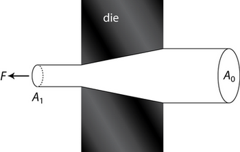
    In wire drawing, a tensile force is applied to the product rather than a compressive force applied to the billet (such as in extrusion for example).
    wire_drawing_sml.png

    To extend the wire by distance \( l_{1} \), we have to feed in a length \( l_{0} \) to the die where \( A_{1} l_{1}=A_{0} l_{0}\) by conservation of volume.

    Work done by \( F=F l_{1} \)

    Volume of metal \( = A_{1} l_{1} \) drawn by \( l_{1} \)

    \[ \text{Work done} =Y A_{1} l_{1} \ln \frac{l_{1}}{l_{0}}=F l_{1} \nonumber \]

    \[ \Rightarrow \frac{F}{A_{1}}=\sigma=Y \ln \frac{l_{1}}{l_{0}}=Y \ln \frac{A_{0}}{A_{1}} \]

    where \( \sigma \) = stress required, the drawing stress.

    Therefore we can estimate the maximum reduction possible with perfect lubrication.

    If there is no work hardening, \( \sigma \leq Y \) then the maximum reduction occurs when

    \[ \sigma=Y \Rightarrow \ln \frac{A_{1}}{A_{0}}=1 \nonumber \]

    \[ \Rightarrow \frac{A_{0}}{A_{1}}=2.72 \]

    (e to 3 s.f.)

    \[ \Rightarrow \frac{A_{1}}{A_{0}}=0.37 \]

    63% is therefore the maximum possible reduction of cross-sectional area with a perfect wire-drawing operation for a rigid-plastic material. Work hardening causes this to increase to a slightly higher value. Friction between the wire and the die reduces this value, causing redundant work – work in excess of the minimum necessary to cause the deformation.

    In practice, the best reduction obtainable with real dies and good lubrication is approximately 50%.

    To allow for redundant work, we can apply empirical corrections, e.g. by using a value of efficiency, \( \eta \):

    \[ \eta=\frac{\text { Work formula estimate }}{\text { Actual total work }} \]

    Typical values of \( \eta \) are:

    • extrusion \( \eta = \) 45 – 55%
    • wire drawing \( \eta = \) 50 – 65%
    • rolling \( \eta = \) 60 – 80%

    Clearly, the work formula method gives a lower band to the true force required for a given deformation processing operation because we are neglecting ‘redundant work.’

    For metalworking, it is often preferable to have an overestimate of the load required in order to be sure that a given operation or process is possible.


    This page titled 1.4: Work Formula Method is shared under a CC BY-NC-SA 2.0 license and was authored, remixed, and/or curated by Dissemination of IT for the Promotion of Materials Science (DoITPoMS) via source content that was edited to the style and standards of the LibreTexts platform.

    • Was this article helpful?