1.3: Slip Line Field Theory
- Page ID
- 7781
\( \newcommand{\vecs}[1]{\overset { \scriptstyle \rightharpoonup} {\mathbf{#1}} } \)
\( \newcommand{\vecd}[1]{\overset{-\!-\!\rightharpoonup}{\vphantom{a}\smash {#1}}} \)
\( \newcommand{\id}{\mathrm{id}}\) \( \newcommand{\Span}{\mathrm{span}}\)
( \newcommand{\kernel}{\mathrm{null}\,}\) \( \newcommand{\range}{\mathrm{range}\,}\)
\( \newcommand{\RealPart}{\mathrm{Re}}\) \( \newcommand{\ImaginaryPart}{\mathrm{Im}}\)
\( \newcommand{\Argument}{\mathrm{Arg}}\) \( \newcommand{\norm}[1]{\| #1 \|}\)
\( \newcommand{\inner}[2]{\langle #1, #2 \rangle}\)
\( \newcommand{\Span}{\mathrm{span}}\)
\( \newcommand{\id}{\mathrm{id}}\)
\( \newcommand{\Span}{\mathrm{span}}\)
\( \newcommand{\kernel}{\mathrm{null}\,}\)
\( \newcommand{\range}{\mathrm{range}\,}\)
\( \newcommand{\RealPart}{\mathrm{Re}}\)
\( \newcommand{\ImaginaryPart}{\mathrm{Im}}\)
\( \newcommand{\Argument}{\mathrm{Arg}}\)
\( \newcommand{\norm}[1]{\| #1 \|}\)
\( \newcommand{\inner}[2]{\langle #1, #2 \rangle}\)
\( \newcommand{\Span}{\mathrm{span}}\) \( \newcommand{\AA}{\unicode[.8,0]{x212B}}\)
\( \newcommand{\vectorA}[1]{\vec{#1}} % arrow\)
\( \newcommand{\vectorAt}[1]{\vec{\text{#1}}} % arrow\)
\( \newcommand{\vectorB}[1]{\overset { \scriptstyle \rightharpoonup} {\mathbf{#1}} } \)
\( \newcommand{\vectorC}[1]{\textbf{#1}} \)
\( \newcommand{\vectorD}[1]{\overrightarrow{#1}} \)
\( \newcommand{\vectorDt}[1]{\overrightarrow{\text{#1}}} \)
\( \newcommand{\vectE}[1]{\overset{-\!-\!\rightharpoonup}{\vphantom{a}\smash{\mathbf {#1}}}} \)
\( \newcommand{\vecs}[1]{\overset { \scriptstyle \rightharpoonup} {\mathbf{#1}} } \)
\( \newcommand{\vecd}[1]{\overset{-\!-\!\rightharpoonup}{\vphantom{a}\smash {#1}}} \)
\(\newcommand{\avec}{\mathbf a}\) \(\newcommand{\bvec}{\mathbf b}\) \(\newcommand{\cvec}{\mathbf c}\) \(\newcommand{\dvec}{\mathbf d}\) \(\newcommand{\dtil}{\widetilde{\mathbf d}}\) \(\newcommand{\evec}{\mathbf e}\) \(\newcommand{\fvec}{\mathbf f}\) \(\newcommand{\nvec}{\mathbf n}\) \(\newcommand{\pvec}{\mathbf p}\) \(\newcommand{\qvec}{\mathbf q}\) \(\newcommand{\svec}{\mathbf s}\) \(\newcommand{\tvec}{\mathbf t}\) \(\newcommand{\uvec}{\mathbf u}\) \(\newcommand{\vvec}{\mathbf v}\) \(\newcommand{\wvec}{\mathbf w}\) \(\newcommand{\xvec}{\mathbf x}\) \(\newcommand{\yvec}{\mathbf y}\) \(\newcommand{\zvec}{\mathbf z}\) \(\newcommand{\rvec}{\mathbf r}\) \(\newcommand{\mvec}{\mathbf m}\) \(\newcommand{\zerovec}{\mathbf 0}\) \(\newcommand{\onevec}{\mathbf 1}\) \(\newcommand{\real}{\mathbb R}\) \(\newcommand{\twovec}[2]{\left[\begin{array}{r}#1 \\ #2 \end{array}\right]}\) \(\newcommand{\ctwovec}[2]{\left[\begin{array}{c}#1 \\ #2 \end{array}\right]}\) \(\newcommand{\threevec}[3]{\left[\begin{array}{r}#1 \\ #2 \\ #3 \end{array}\right]}\) \(\newcommand{\cthreevec}[3]{\left[\begin{array}{c}#1 \\ #2 \\ #3 \end{array}\right]}\) \(\newcommand{\fourvec}[4]{\left[\begin{array}{r}#1 \\ #2 \\ #3 \\ #4 \end{array}\right]}\) \(\newcommand{\cfourvec}[4]{\left[\begin{array}{c}#1 \\ #2 \\ #3 \\ #4 \end{array}\right]}\) \(\newcommand{\fivevec}[5]{\left[\begin{array}{r}#1 \\ #2 \\ #3 \\ #4 \\ #5 \\ \end{array}\right]}\) \(\newcommand{\cfivevec}[5]{\left[\begin{array}{c}#1 \\ #2 \\ #3 \\ #4 \\ #5 \\ \end{array}\right]}\) \(\newcommand{\mattwo}[4]{\left[\begin{array}{rr}#1 \amp #2 \\ #3 \amp #4 \\ \end{array}\right]}\) \(\newcommand{\laspan}[1]{\text{Span}\{#1\}}\) \(\newcommand{\bcal}{\cal B}\) \(\newcommand{\ccal}{\cal C}\) \(\newcommand{\scal}{\cal S}\) \(\newcommand{\wcal}{\cal W}\) \(\newcommand{\ecal}{\cal E}\) \(\newcommand{\coords}[2]{\left\{#1\right\}_{#2}}\) \(\newcommand{\gray}[1]{\color{gray}{#1}}\) \(\newcommand{\lgray}[1]{\color{lightgray}{#1}}\) \(\newcommand{\rank}{\operatorname{rank}}\) \(\newcommand{\row}{\text{Row}}\) \(\newcommand{\col}{\text{Col}}\) \(\renewcommand{\row}{\text{Row}}\) \(\newcommand{\nul}{\text{Nul}}\) \(\newcommand{\var}{\text{Var}}\) \(\newcommand{\corr}{\text{corr}}\) \(\newcommand{\len}[1]{\left|#1\right|}\) \(\newcommand{\bbar}{\overline{\bvec}}\) \(\newcommand{\bhat}{\widehat{\bvec}}\) \(\newcommand{\bperp}{\bvec^\perp}\) \(\newcommand{\xhat}{\widehat{\xvec}}\) \(\newcommand{\vhat}{\widehat{\vvec}}\) \(\newcommand{\uhat}{\widehat{\uvec}}\) \(\newcommand{\what}{\widehat{\wvec}}\) \(\newcommand{\Sighat}{\widehat{\Sigma}}\) \(\newcommand{\lt}{<}\) \(\newcommand{\gt}{>}\) \(\newcommand{\amp}{&}\) \(\definecolor{fillinmathshade}{gray}{0.9}\)This approach is used to model plastic deformation in plane strain only for a solid that can be represented as a rigid-plastic body. Elasticity is not included and the loading has to be quasi-static. In terms of applications, the approach now has been largely superseded by finite element modelling, as this is not constrained in the same way and for which there are now many commercial packages designed for complex loading (including static and dynamic forces plus temperature variations). Nonetheless, slip line field theory can provide analytical solutions to a number of metal forming processes, and utilizes plots showing the directions of maximum shear stress in a rigid-plastic body which is deforming plastically in plane strain. These plots show anticipated patterns of plastic deformation from which the resulting stress and strain fields can be estimated.
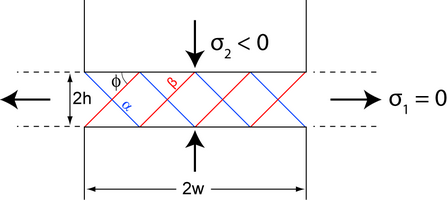
The earlier analysis of plane strain plasticity in a simple case of uniaxial compression established the basis of slip line field theory, which enables the directions of plastic flow to be mapped out in plane strain plasticity problems.
There will always be two perpendicular directions of maximum shear stress in a plane. These generate two orthogonal families of slip lines called α-lines and β-lines. (Labelling convention for α and β lines.)

Experimentally, these lines can be seen in a realistic plastic deformation situation, e.g.
- Polyvinyl chloride (PVC) viewed between crossed polars
- Nitrogen-containing steels can be etched using Fry’s reagent to reveal regions of plastic flow in samples such as notched bars and thick walled cylinders.
- Under dull red heat in forging, we see a distinct red cross caused by dissipation of mechanical energy on slip planes.
To develop slip line field theory to more general plane strain conditions, we need to recognize that the stress can vary from point to point.
Therefore, p can vary, but k is a material constant. As a result of this, directions of maximum shear stress and the directions of principal stresses can vary along a slip line.
Hencky relations
These equations arise from consideration of the equilibrium equations in plane strain.
\[ \begin{array}{l}{p+2 k \varphi=\text { constant along an } \alpha \text { line }} \\ {p-2 k \varphi=\text { constant along a } \beta \text { line }}\end{array} \nonumber \]
 Click here for the derivation.
We can apply these relations to the classic problem of indentation of a material by a flat punch. This is important in hardness testing, in foundations of buildings and in forging.
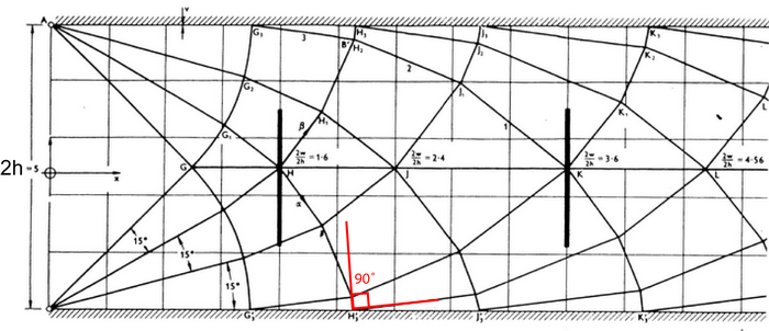
In more general cases, slip lines do not intersect external boundaries at 45° because of friction. In the extreme case, sticking friction occurs (a perfectly rough surface) and slip lines are at 90° to the surface.

Slip-line field for compression between a pair of rough parallel platens [1]
The slip line patterns above are very useful for analyzing plane strain deformation in a rigid-plastic isotropic solid. Arrival at this slip-line pattern is rather complex. They are either derived from model experiments in which the slip-line field is apparent or they are postulated from experience of problems with similar geometry.
For a slip line to be a valid solution (but not necessarily a unique solution) the stress distribution throughout the whole body, not just in the plastic region, must not violate stress equilibrium nor must it violate the yield criterion outside the slip-line field.
The resultant velocity field must also be evaluated to ensure that strain compatibility is satisfied and matter is conserved.
These are stringent conditions and mean that obtaining a slip-line field solution is often not simple.
Instead, it is useful to take a more simple approach to analysing deformation processing operations where one or another of the stringent conditions are relaxed to give useful approximate solutions for part of the analysis.


