11.6: Analysis of Indeterminate Frames

Indeterminate frames are categorized as frames with or without side-sway. A frame with side-sway is one that permits a lateral moment or a swaying to one side due to the asymmetrical nature of its structure or loading. The analysis of frames without side-sway is similar to the analysis of beams considered in the preceding section, while the analysis of frames with side-sway requires taking into consideration the effect of the lateral movement of the structure.

Analysis of Frames with Side-Sway

Consider the frame shown in Figure 11.6 for an illustration of the effect of side-sway on a frame. Due to the asymmetrical application of the loads, there will be a lateral displacement \(\Delta\) to the right at \(B\) and \(C\), which subsequently will cause chord rotations \(\psi_{A B}\left(\frac{\Delta}{L_{A B}}\right)\) and \(\psi_{D C}\left(\frac{\Delta}{L_{D C}}\right)\) in columns \(AB\) and \(DC\), respectively. These rotations must be considered when writing the slope-deflection equations for the columns, as will be demonstrated in the solved examples.

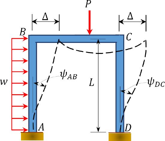
\(Fig. 11.6\). Frame.

Example 11.1

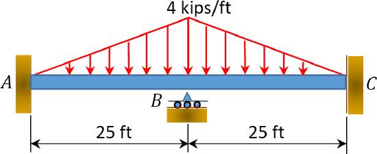
Using the slope-deflection method, determine the end moments and the reactions at the supports of the beam shown in Figure 11.7a and draw the shearing force and the bending moment diagrams. \(EI\) = constant.

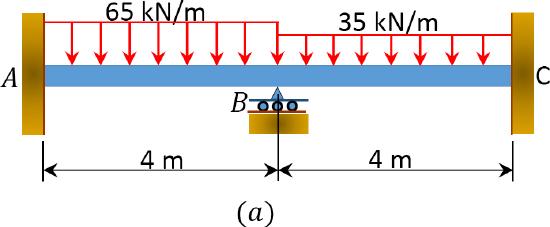
\(Fig. 11.7\). Beam.

Solution

Fixed-end moments.

The Fixed-end moments (FEM) using Table 11.1 are computed as follows:

\(\begin{array}{l}
F E M_{A B}=-\frac{w \mathrm{~L}^{2}}{12}=-\frac{65 \times 4^{2}}{12}=-86.67 \mathrm{kN} . \mathrm{m} \\
F E M_{B A}=\frac{w \mathrm{~L}^{2}}{12}=86.67 \mathrm{kN} . \mathrm{m} \\
F E M_{B C}=-\frac{35 \times 4^{2}}{12}=-46.67 \mathrm{kN} . \mathrm{m} \\
F E M_{C B}=46.67 \mathrm{kN} . \mathrm{m}
\end{array}\)

Slope-deflection equations. As \(\delta_{A} = \delta_{C} = 0\) due to fixity at both ends and \(\psi_{A B}=\psi_{B C}=0\) as no settlement occurs, equations for member end moments are expressed as follows:

\[\begin{array}{c}
M_{A B}=\frac{2 \mathrm{EI}}{L}\left(2 \theta_{A}+\theta_{B}-3 \psi\right)+F E M_{A B} \\
2 \mathrm{EK} \theta_{B}-86.67
\end{array}\]

\[\begin{array}{c}
M_{B A}=\frac{2 \mathrm{EI}}{L}\left(\theta_{A}+2 \theta_{B}-3 \psi\right)+F E M_{B A} \\
4 \mathrm{EK} \theta_{B}+86.67
\end{array}\]

\[\begin{array}{c}
M_{B C}=\frac{2 \mathrm{EI}}{L}\left(2 \theta_{B}+\theta_{C}-3 \psi\right)+F E M_{B C} \\
4 \mathrm{EK} \theta_{B}-46.67
\end{array}\]

\[\begin{array}{c}
M_{C B}=\frac{2 \mathrm{EI}}{L}\left(\theta_{B}+2 \theta_{C}-3 \psi\right)+F E M_{C B} \\
2 \mathrm{EK} \theta_{B}+46.67
\end{array}\]

Joint equilibrium equation.

Equilibrium equation at joint \(B\) is as follows:

\(\begin{array}{l}
\sum \mathrm{M}_{B}=\mathrm{M}_{B A}+\mathrm{M}_{B C}=0 \\
4 \mathrm{EK} \theta_{B}+86.67+4 \mathrm{EK} \theta_{B}-46.67=0 \\
\theta_{B}=-\frac{5}{\mathrm{EK}}
\end{array}\)

Final end moments.

Substituting \(\theta_{B}=-\frac{5}{\mathrm{EK}}\) into equations 1, 2, 3, and 4 suggests the following:

\(\begin{array}{l}
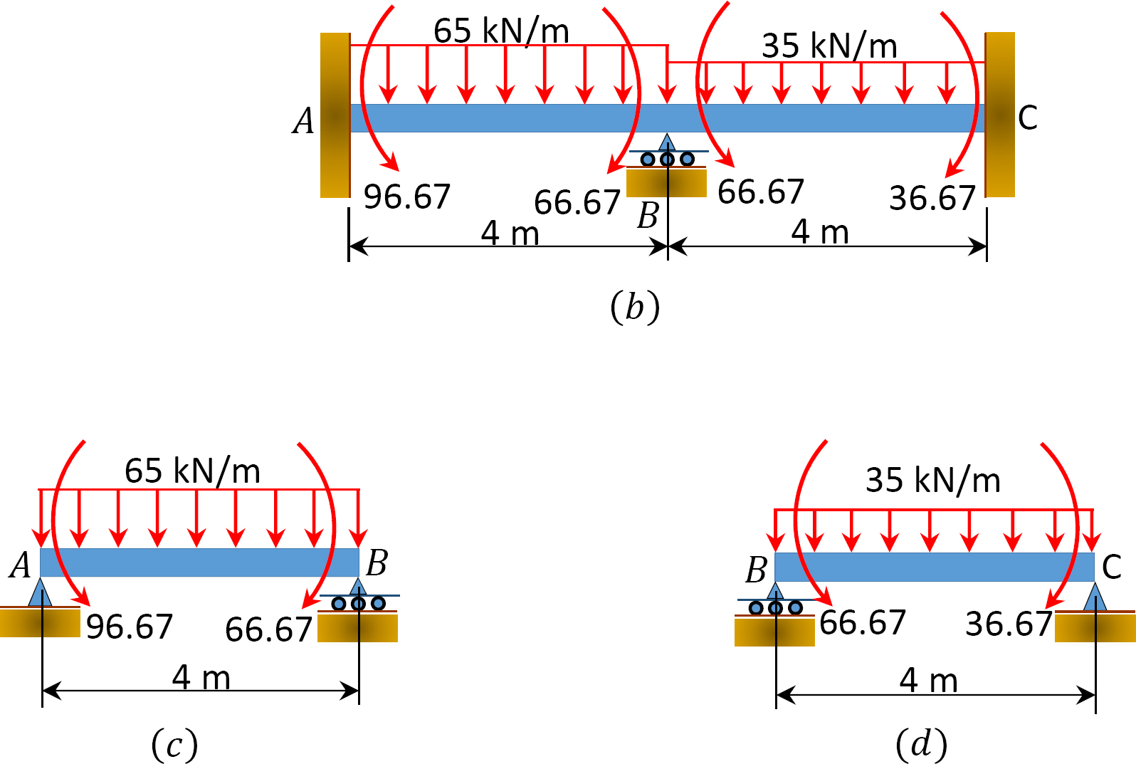
M_{A B}=2 \mathrm{EK}\left(-\frac{5}{\mathrm{EK}}\right)-86.67=-96.67 \mathrm{kN} . \mathrm{m} \\
M_{B A}=4 \mathrm{EK}\left(-\frac{5}{\mathrm{EK}}\right)+86.67=66.67 \mathrm{kN} . \mathrm{m} \\
M_{B C}=4 \mathrm{EK}\left(-\frac{5}{\mathrm{EK}}\right)-46.67=-66.67 \mathrm{kN} . \mathrm{m} \\
M_{C B}=2 \mathrm{EK}\left(-\frac{5}{\mathrm{EK}}\right)+46.67=36.67 \mathrm{kN} . \mathrm{m}
\end{array}\)

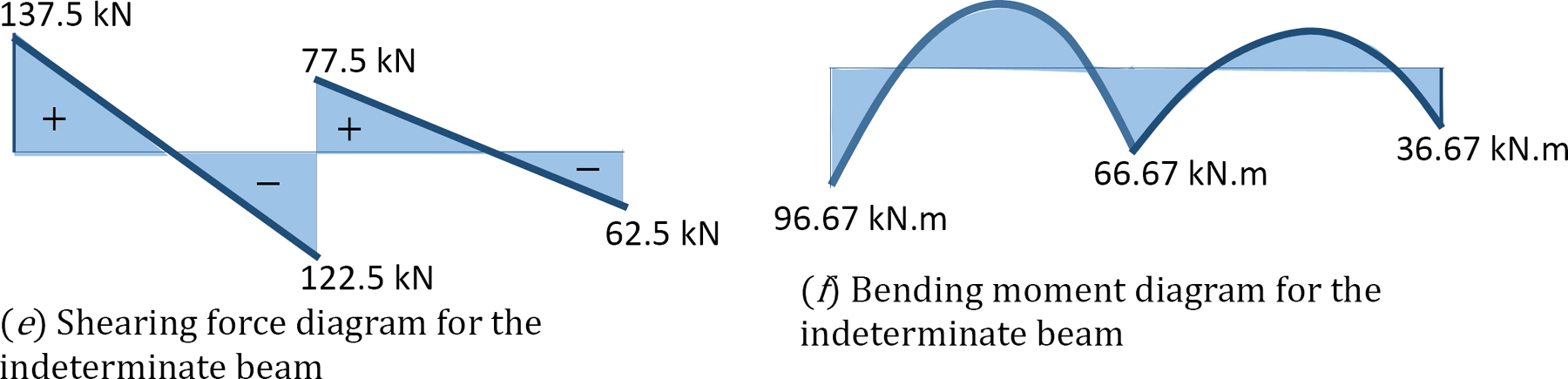
Shearing force and bending moment diagrams.

Shear force and bending moment for segment \(AB\).

First compute the reaction at support \(A\), as follows:

\(\begin{array}{l}
\curvearrowleft +\sum M_{B}=0:-4 A_{y}+96.67+(65)(4)(2)-66.67=0 \\
A_{y}=137.5 \mathrm{kN}
\end{array}\)

Calculate the shear force, as follows:

 

When \(x = 0\), \(V=137.5 \mathrm{kN}\)

When \(x = 4 \mathrm{m}\), \(V=-122.5 \mathrm{kN}\)

Find the moment, as follows:

\(M=137.5 x-\frac{(65)(x)^{2}}{2}-96.67\)

When \(x = 0\), \(M=-96.67 \mathrm{kN} . \mathrm{m}\)

When \(x = 4\) m, \(M=-66.67 \mathrm{kN} . \mathrm{m}\)

Shear force and bending moment for segment \(AB\).

First determine the reaction at \(B\), as follows:

\(\begin{array}{l}
\curvearrowleft +\sum M_{C}=0:-4 B_{y}+66.67+(35)(4)(2)-36.67=0 \\
B_{y}=77.5 \mathrm{kN}
\end{array}\)

Calculate the shear force, as follows:

 

When \(x = 0\), \(V=77.5 \mathrm{kN}\).

When \(x = 4\) m, \(V=-62.5 \mathrm{kN}\).

Find the moment, as follows:

\(M=77.5 x-\frac{(35)(x)^{2}}{2}-66.67\)

When \(x = 0\), \(M=-66.67 \mathrm{kN} . \mathrm{m}\)

When \(x = 4\) m, \(M=-36.67 \mathrm{kN} . \mathrm{m}\)

Shear force and bending moment diagrams.

Example 11.2

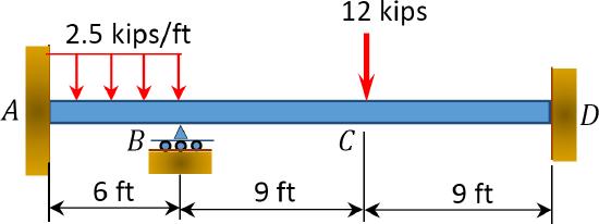
Using the slope-deflection method, determine the end moments and the reactions at the supports of the beam shown in Figure 11.8a, and draw the shearing force and the bending moment diagrams. \(EI\) = constant.

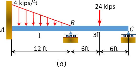
\(Fig. 11.8\). Beam.

Solution

Relative stiffness.

\(\left(K_{A B}\right):\left(K_{B C}\right)=\left(\frac{1}{12}\right):\left(\frac{3 I}{12}\right)=1: 3\)

Fixed-end moments.

\(\begin{array}{l}
F E M_{A B}=-\frac{w \mathrm{~L}^{2}}{20}=-\frac{(4)(12)^{2}}{20}=-28.8 \mathrm{k} . \mathrm{ft} \\
F E M_{B A}=\frac{w \mathrm{~L}^{2}}{30}=\frac{(4)(12)^{2}}{30}=19.2 \mathrm{k} . \mathrm{ft} \\
F E M_{B C}=-\frac{\mathrm{PL}}{8}=-\frac{24 \times 12}{8}=-36 \mathrm{k} . \mathrm{ft} \\
F E M_{C B}=\frac{\mathrm{PL}}{8}=36 \mathrm{k} . \mathrm{ft}
\end{array}\)

Slope-deflection equations.

Noting that \(M_{C B}=\psi=0\), equations for member end moments can be expressed as follows: \[\begin{aligned}
M_{A B} &=(2)(1)\left(2 \theta_{A}+\theta_{B}-3 \psi\right)+F E M_{A B} \\
&=2 \theta_{B}-28.8
\end{aligned}\]

\[\begin{aligned}
M_{B A} &=(2)(1)\left(\theta_{A}+2 \theta_{B}-3 \psi\right)+F E M_{B A} \\
&=4 \theta_{B}+19.2
\end{aligned}\]

\[\begin{aligned}
M_{B C} &=3(3)\left(\theta_{B}-\psi\right)+F E M_{B C}-\frac{F E M_{C B}}{2} \\
&=3(3) \theta_{B}-36-\frac{36}{2} \\
&=9 \theta_{B}-54
\end{aligned}\]

Joint equilibrium equation.

The equilibrium equation at joint \(B\) is as follows:

\(\begin{array}{c}
\sum M_{B}=M_{B A}+M_{B C}=0 \\
4 \theta_{B}+19.2+9 \theta_{B}-54=0 \\
\theta_{B}=\frac{34.8}{13}=2.68
\end{array}\)

Final end moments.

Substituting the computed value of \(\theta_{B}\) into equations 1, 2, and 3 suggests the following:

\(\begin{array}{l}
M_{A B}=2(2.68)-28.8=-23.4 \mathrm{k} . \mathrm{ft} \\
M_{B A}=4 \theta_{B}+19.2=4(2.68)+19.2=29.9 \mathrm{k} . \mathrm{ft} \\
M_{B C}=9 \theta_{B}-54=9(2.68)-54=-29.9 \mathrm{k.} \mathrm{ft} \\
M_{C B}=0
\end{array}\)

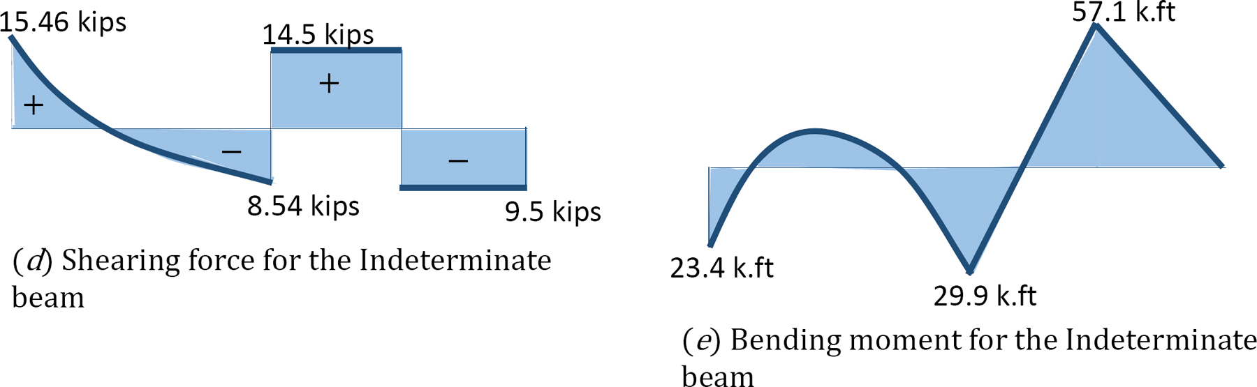
Shear force and bending moment diagrams.

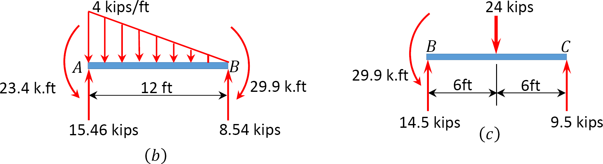
Shear force and bending moment for segment \(AB\).

\(\begin{aligned}
\curvearrowleft +& \sum M_{A}=0: 12 B_{y}+23.44-\left(\frac{1}{2}\right)(12)(4)\left(\frac{1}{3} \times 12\right)-29.9=0 \\
B_{y} &=8.54 \mathrm{kips} \\
\uparrow+\sum F_{y}=& 8.54+A_{y}-\left(\frac{1}{2}\right)(12)(4)=0 \\
A_{y} &=15.46 \mathrm{kips} \\
V &=-8.54+\left(\frac{1}{2}\right)(x)\left(\frac{x}{3}\right)=-8.54+\frac{x^{2}}{6}
\end{aligned}\)

When \(x = 0\), \(V=-8.54 \mathrm{kips}\)

When \(x = 12\) ft, \(V=15.46 \mathrm{kips}\)

\(M=8.54 x-\left(\frac{1}{2}\right)(x)\left(\frac{x}{3}\right)\left(\frac{1}{3} \times x\right)-29.9=8.54 x-\frac{(x)^{3}}{18}-29.9\)

When \(x = 0\), \(M=-29.9 \mathrm{k} . \mathrm{ft}\)

When \(x = 12\)ft, \(M=-23.4 \mathrm{k} . \mathrm{ft}\)

Shear force and bending moment for segment \(BC\).

\(\begin{array}{l}
\curvearrowleft +\sum M_{B}=0: 12 C_{y}+29.9-(24)(6)=0 \\
C_{y}=9.5 \mathrm{kips} \\
\uparrow+\sum F_{y}=0
\end{array}\)

\(\begin{aligned}
&B_{y}+9.5-24=0\\
&B_{y}=14.5 \mathrm{kips}\\
&0<x<6 \mathrm{ft}\\
&V=14.5 \text { kips }\\
&M=14.5 x-29.9\\
&\text { When } x=0, M=-29.9 \mathrm{k} . \mathrm{ft}\\
&\text { When } x=6 \mathrm{ft}, M=57.10 \mathrm{k} . \mathrm{ft}
\end{aligned}\)

Example 11.3

Using the slope-deflection method, determine the end moments of the beam shown in Figure 11.9a. Assume support \(B\) settles 1.5 in, and draw the shear force and the bending moment diagrams. The modulus of elasticity and the moment of inertia of the beam are \(29,000 \mathrm{ksi}\) and \(8000 \mathrm{in}^{4}\), respectively.

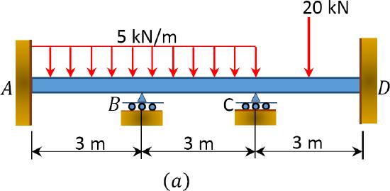
\(Fig. 11.9\). Beam.

Solution

Fixed-end moments.

The Fixed-end moments (FEM) using Table 11.1 are computed as follows:

\(\begin{array}{l}
F E M_{A B}=-\frac{w L^{2}}{12}=-\frac{5 \times 3^{2}}{12}=-3.75 \mathrm{kN} . \mathrm{m} \\
F E M_{B A}=\frac{w \mathrm{~L}^{2}}{12}=3.75 \mathrm{kN} . \mathrm{m} \\
F E M_{B C}=-3.75 \mathrm{kN} . \mathrm{m} \\
F E M_{C B}=3.75 \mathrm{kN} . \mathrm{m} \\
F E M_{C D}=-\frac{\mathrm{Pab}^{2}}{L^{2}}=\frac{(20)(1.5)(1.5)^{2}}{3^{2}}=-7.5 \mathrm{kN} . \mathrm{m} \\
F E M_{D C}=\frac{\mathrm{P} a^{2} \mathrm{~b}}{L^{2}}=\frac{(20)(1.5)(1.5)^{2}}{3^{2}}=7.5 \mathrm{kN} \cdot \mathrm{m}
\end{array}\)

Slope-deflection equations.

At \(\theta_{A}=\theta_{D}=\psi=0\), the equations for member end moments are expressed as follows: \[\begin{aligned}
M_{A B} &=\frac{2 \mathrm{EI}}{L}\left(2 \theta_{A}+\theta_{B}-3 \psi\right)-F E M_{A B} \\
=& 2 \mathrm{EK} \theta_{B}-3.75
\end{aligned}\]

\[\begin{aligned}
M_{B A} &=\frac{2 \mathrm{EI}}{L}\left(\theta_{A}+2 \theta_{B}-3 \psi\right)+F E M_{B A} \\
&=4 \mathrm{EK} \theta_{B}+3.75
\end{aligned}\]

\[\begin{aligned}
M_{B C} &=\frac{2 E I}{L}\left(2 \theta_{B}+\theta_{C}-3 \psi\right)-F E M_{B C} \\
=& 4 \mathrm{EK} \theta_{B}+2 \mathrm{EK} \theta_{C}-3.75
\end{aligned}\]

\[\begin{aligned}
\mathrm{M}_{C B}=& \frac{2 \mathrm{EI}}{L}\left(\theta_{B}+2 \theta_{C}-3 \psi\right)+\mathrm{FEM}_{C B} \\
=2 \mathrm{EK} \theta_{B}+4 \mathrm{EK} \theta_{C}+3.75 &
\end{aligned}\]

\[\begin{aligned}
\mathrm{M}_{C D}=\frac{2 \mathrm{EI}}{L}\left(2 \theta_{C}+\theta_{D}-3 \psi\right)-\mathrm{FEM}_{C D} \\
=4 \mathrm{EK} \theta_{c}-7.5
\end{aligned}\]

\[\begin{aligned}
\mathrm{M}_{D C}=\frac{2 \mathrm{EI}}{L}\left(\theta_{C}+2 \theta_{D}-3 \psi\right)+\mathrm{FEM}_{D C} \\
=2 \mathrm{EK} \theta_{C}+7.5
\end{aligned}\]

Joint equilibrium equation.

The equilibrium equation at joint \(B\) is as follows: \[\begin{array}{l}
\qquad \sum M_{B}=M_{B A}+M_{B C}=0 \\
4 E K \theta_{B}+3.75+4 E K \theta_{B}+2 E K \theta_{C}-3.75=0 \\
8 E K \theta_{B}+2 E K \theta_{C}=0
\end{array}\]

\[\begin{array}{l}
\sum M_{C}=M_{C B}+M_{C D}=0 \\
2 E K \theta_{B}+4 E K \theta_{C}+3.75+4 E K \theta_{C}-7.5=0 \\
2 E K \theta_{B}+8 E K \theta_{C}-3.75=0
\end{array}\]

Solving equations 7 and 8 simultaneously suggests the following:

\(\theta_{B}=-\frac{0.125}{\mathrm{EK}} \text { and } \theta_{C}=\frac{0.5}{\mathrm{EK}}\)

Final end moments.

Substituting the obtained values of \(\theta_{B}\) and \(\theta_{C}\) into the slope-deflection equations suggests the following end moments:

\(\begin{array}{l}
M_{A B}=2 E K\left(-\frac{0.125}{\mathrm{EK}}\right)-3.75=-4.00 \mathrm{kN} . \mathrm{m} \\
M_{B A}=4 E K\left(-\frac{0.125}{\mathrm{EK}}\right)+3.75=3.25 \mathrm{kN} . \mathrm{m} \\
M_{B C}=4 \mathrm{EK}\left(\frac{0.125}{\mathrm{EK}}\right)+2(0.5)-3.75=-3.25 \mathrm{kN} . \mathrm{m} \\
M_{C B}=2 \mathrm{EK}\left(-\frac{0.125}{\mathrm{EK}}\right)+4(0.5)+3.75=5.50 \mathrm{kN} . \mathrm{m} \\
M_{C D}=4 \mathrm{EK}\left(-\frac{0.5}{\mathrm{EK}}\right)-7.5=-5.50 \mathrm{kN} . \mathrm{m} \\
M_{D C}=2 \mathrm{EK}\left(-\frac{0.5}{\mathrm{EK}}\right)+7.5=8.5 \mathrm{kN} . \mathrm{m}
\end{array}\)

Example 11.4

Using the slope-deflection method, determine the member end moments of the beam of the rectangular cross section shown in Figure 11.10a. Assume that support \(B\) settles 2 cm. The modulus of elasticity and the moment of inertia of the beam are \(E=210,000 \mathrm{~N} / \mathrm{mm}^{2}\) and \(4.8 \times 10^{4} \mathrm{~mm}^{4}\), respectively.

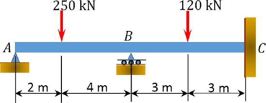
\(Fig. 11.10\). Rectangular cross section of beam.

Solution

The Fixed-end moments (FEM) using Table 11.1 are computed as follows:

\(\begin{array}{l}
F E M_{A B}=-\frac{P a b^{2}}{L^{2}}=-\frac{(250)(2)(4)^{2}}{6^{2}}=-222.22 \mathrm{kN} . \mathrm{m} \\
F E M_{B A}=\frac{P a^{2} b}{L^{2}}=\frac{(250)(2)^{2}(4)}{6^{2}}=111.1 \mathrm{kN} . \mathrm{m} \\
F E M_{B C}=-\frac{P L}{8}=-\frac{(120)(6)}{8}=-90 \mathrm{kN} . \mathrm{m} \\
F E M_{C B}=\frac{P L}{8}=\frac{(120)(6)}{8}=90 \mathrm{kN} . \mathrm{m}
\end{array}\)

Slope-deflection equations.

As \(\theta_{C}=0\), equations for member end moments are expressed as follows: \[\begin{aligned}
M_{B A} &=3 E K\left(\theta_{B}-\Psi\right)+F E M_{B A}-\frac{F E M_{A B}}{2} \\
&=3 E K\left(\theta_{B}-\frac{0.02}{6}\right)+111.1-\frac{(-222.2)}{2} \\
&=3 E K \theta_{B}-0.01 E K+222.2
\end{aligned}\]

\[\begin{aligned}
M_{B C} &=2 E K\left(2 \theta_{B}+\theta_{C}-3 \psi\right)+F E M_{B C} \\
&=4 E K \theta_{B}+2 E K\left(-3 \times \frac{(-0.02)}{6}\right)-90 \\
&=4 E K \theta_{B}+0.02 E K-90
\end{aligned}\]

\[\begin{aligned}
M_{C B} &=2 E K\left(\theta_{B}+2 \theta_{C}-3 \psi\right)+F E M_{C B} \\
&=2 E K \theta_{B}+0.02 E K+90
\end{aligned}\]

Joint equilibrium equation.

The equilibrium equation at joint \(B\) is written as follows: \[\begin{array}{l}
\qquad \sum M_{B}=M_{B A}+M_{B C}=0 \\
3 E K \theta_{B}-0.01 E K+222.2+4 E K \theta_{B}+0.02 E K-90=0 \\
7 E K \theta_{B}+0.01 E K+132.2=0
\end{array}\]

Solving equation 4 for \(\theta_{B}\) suggests the following:

\(\begin{array}{l}
\theta_{B}=-0.0014-\frac{18.89}{E K}=-0.0014-\frac{18.89}{210 \times 10^{9} K} \\
E K=210 \times 10^{9} \times \frac{4.8 \times 10^{4}}{\left(10^{12}\right)(6)}=1680 \\
\theta_{B}=-0.0014-\frac{18.89}{1680}=-0.0126 \mathrm{rad}
\end{array}\)

Final end moments.

Substituting the obtained value of \(\theta_{B}\) into equations 1, 2, and 3 suggests the following end moments:

\(\begin{array}{l}
M_{A B}=0 \\
\qquad M_{B A}=141.9 \mathrm{kN} \cdot \mathrm{m} \\
M_{B C}=4 E K\left(\frac{0.125}{E K}\right)+2(0.5)-3.75=-141.07 \mathrm{kN} . \mathrm{m} \\
M_{C B}=2 E K\left(-\frac{0.125}{E K}\right)+4(0.5)+3.75=81.26 \mathrm{kN} . \mathrm{m}
\end{array}\)

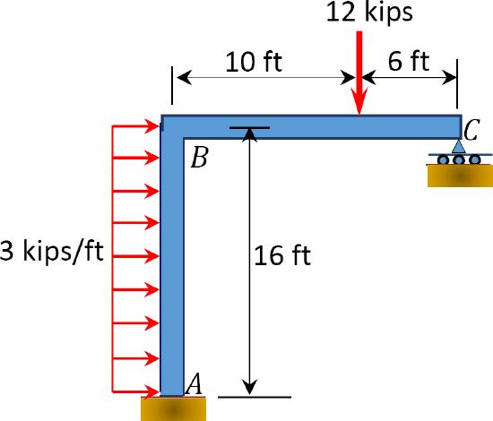
Example 11.5

Using the slope-deflection method, determine the member end moments and the reactions at the supports of the frame shown in Figure 11.11a. \(EI =\) constant.

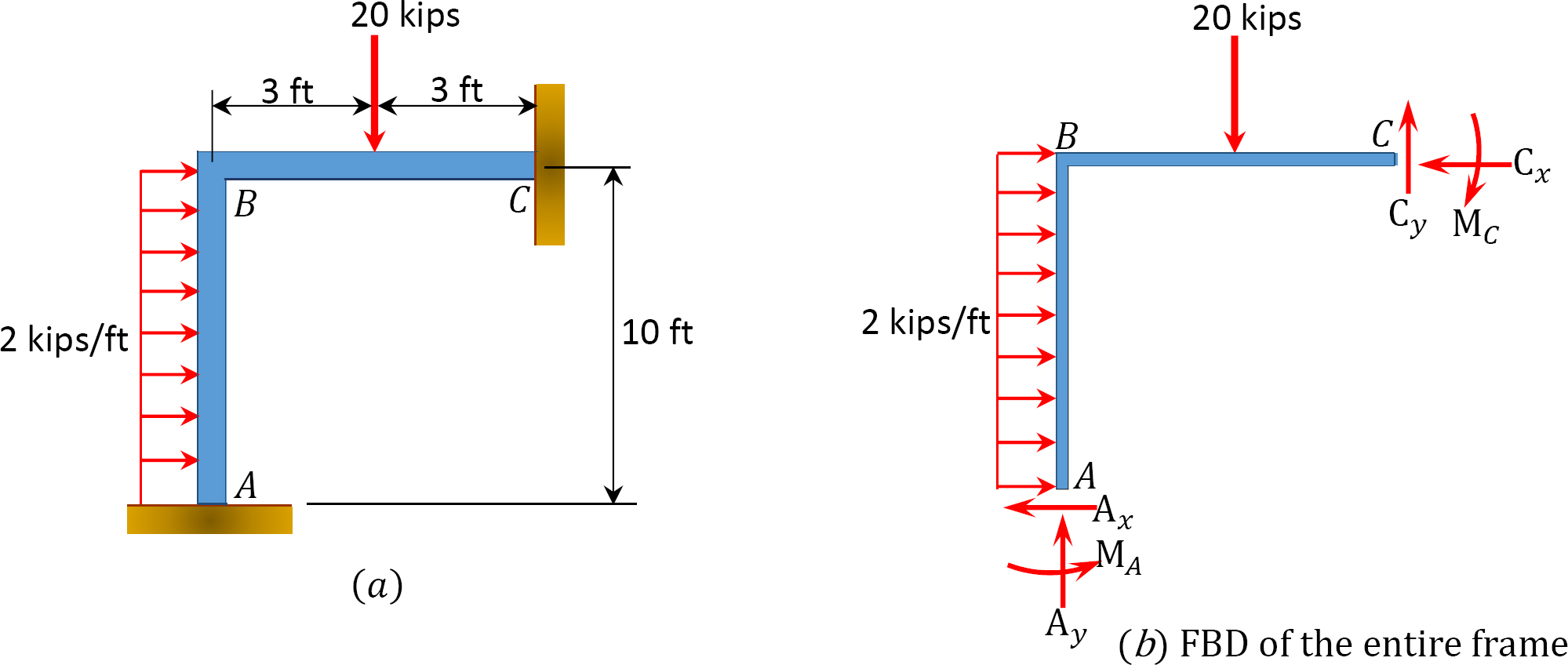
\(Fig. 11.11\). Frame.

Solution

Fixed-end moments.

The Fixed-end moments (FEM) using Table 11.1 are computed as follows:

\(\begin{array}{l}
F E M_{A B}=-\frac{w \mathrm{~L}^{2}}{12}=-\frac{2 \times 10^{2}}{12}=-16.67 \mathrm{k} . \mathrm{ft} \\
F E M_{B A}=\frac{w L^{2}}{12}=16.67 \mathrm{k} . \mathrm{ft} \\
F E M_{B C}=-\frac{P L}{8}=-\frac{20 \times 6}{8}=-15 \\
F E M_{C B}=\frac{P L}{8}=\frac{20 \times 6}{8}=15
\end{array}\)

Slope-deflection equations.

As \(\theta_{A}=\theta_{C}=0\) due to fixity at both ends and \(\psi_{A B}=\psi_{B C}=0\) since no settlement occurs, equations for the member end moments are expressed as follows: \[\begin{aligned}
M_{A B} &=2 E K\left(2 \theta_{A}+\theta_{B}-3 \psi\right)+F E M_{A B} \\
=2 E K \theta_{B}-16.67 &
\end{aligned}\]

\[\begin{aligned}
M_{B A} &=2 E K\left(\theta_{A}+2 \theta_{B}-3 \psi\right)+F E M_{B A} \\
=4 E K \theta_{B}+16.67 &
\end{aligned}\]

\[\begin{aligned}
& M_{B C}=2 E K\left(2 \theta_{B}+\theta_{C}-3 \psi\right)+F E M_{B C} \\
=4 E K \theta_{B}-15 &
\end{aligned}\]

\[\begin{aligned}
M_{C B} &=\frac{2 E 1}{L}\left(\theta_{B}+2 \theta_{C}-3 \psi\right)+F E M_{C B} \\
=2 E K \theta_{B}+15 &
\end{aligned}\]

Joint equilibrium equation.

The equilibrium equation at joint \(B\) is as follows:

\(\begin{array}{l}
\sum M_{B}=M_{B A}+M_{B C}=0 \\
4 E K \theta_{B}+16.67+4 E K \theta_{B}-15=0 \\
\qquad E K \theta_{B}=-\frac{1.67}{8}=-0.209
\end{array}\)

Final end moments.

Substituting \(E K \theta_{B}=-0.209\) into equations 1, 2, 3, and 4 suggests the following:

\(\begin{array}{l}
M_{A B}=-17.09 \mathrm{k} . \mathrm{ft} \\
M_{B A}=15.83 \mathrm{k.ft} \\
M_{B C}=-15.83 \mathrm{k.ft} \\
M_{C B}=14.58 \mathrm{k.ft}
\end{array}\)

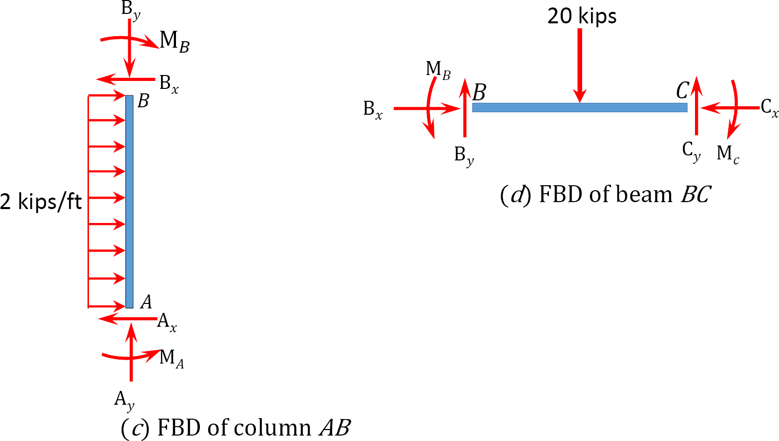
Reactions at supports.

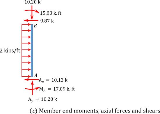
To determine \(A_{x}\), take the moment about \(B\) in Figure 11.11c, as follows:

\(\begin{array}{l}
+\curvearrowleft \Sigma M_{B}=0: 17.09+(2)(10)(5)-15.83-10 A_{x}=0 \\
A_{x}=10.13 \mathrm{k}
\end{array}\)

To determine \(A_{y}\), take the moment about \(C\) in Figure 11.11b, as follows:

\(\begin{array}{l}
+\curvearrowleft \sum M_{C}=0 ; 17.09-10.13 \times 10+(2)(10)(5)+20 \times 3-14.58-6 A_{y}=0 \\
A_{y}=10.20 \mathrm{k}
\end{array}\)

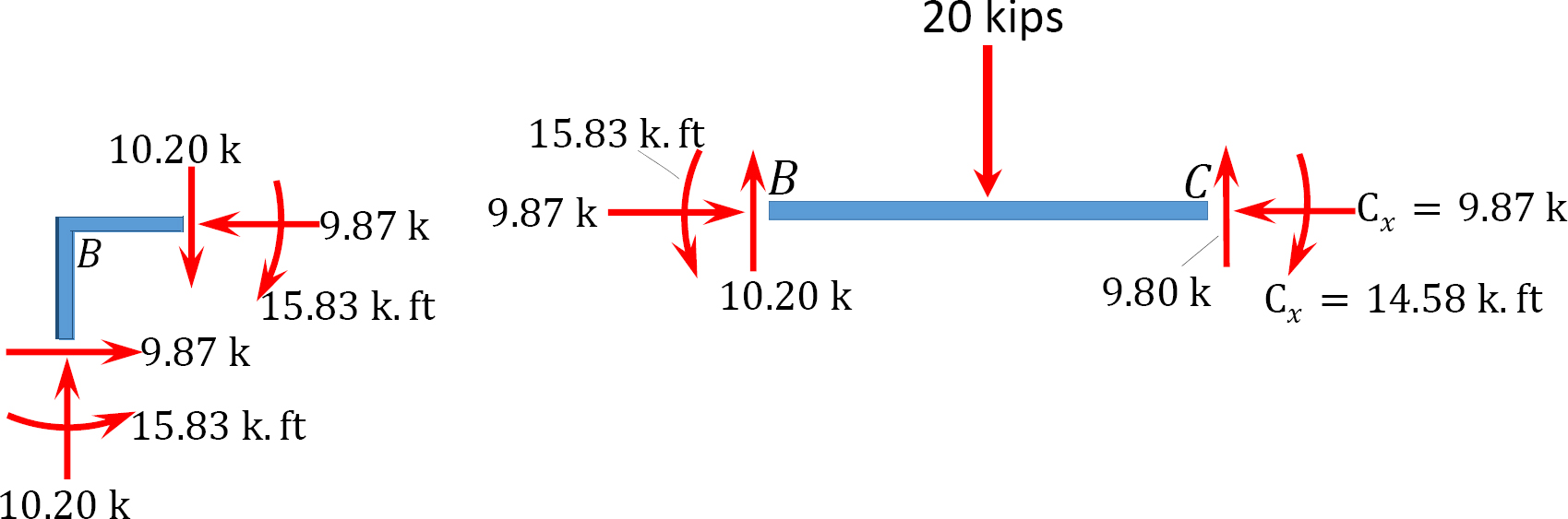
To determine \(C_{y}\) in Figure 11.11b, consider the summation of forces in the vertical direction, as follows:

\(\begin{array}{l}
+\uparrow \sum F_{y}=0 \\
10.20-20+C_{y}=0 \\
C_{y}=9.80 \mathrm{k}
\end{array}\)

To determine \(C_{x}\) in Figure 11.11b, consider the summation of forces in the horizontal direction, as follows:

\(\begin{array}{l}
+\rightarrow \sum F_{x}=0 \\
2 \times 10-10.13-C_{x}=0 \\
C_{x}=9.87 \mathrm{k}
\end{array}\)

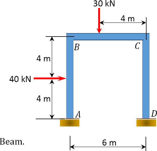
Example 11.6

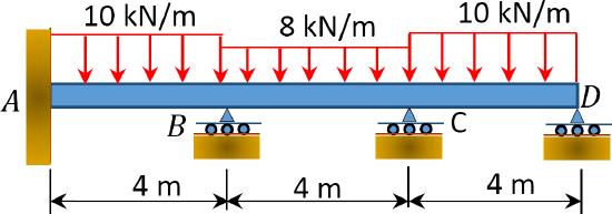
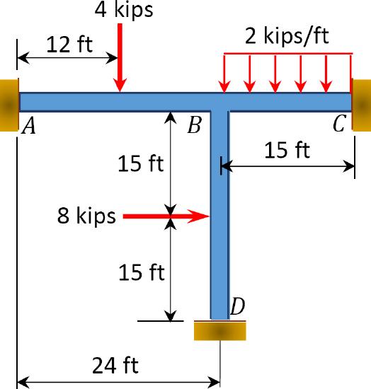
Using the slope-deflection method, determine the member end moments of the frame shown in Figure 11.12a.

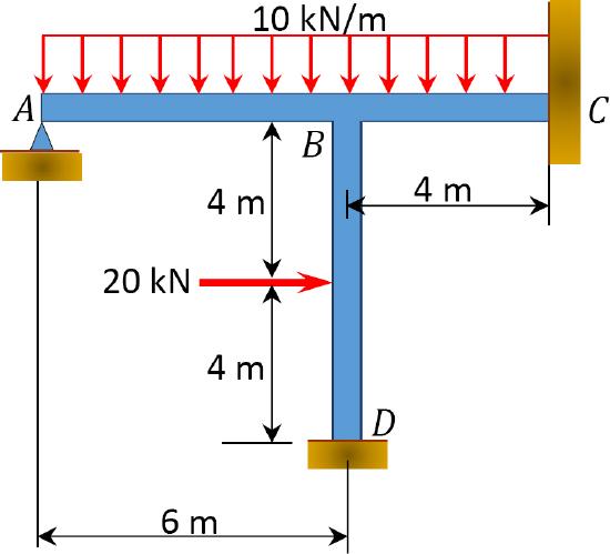
\(Fig. 11.12\). Frame.

Solution

Fixed-end moments.

The Fixed-end moments (FEM) using Table 11.1 are computed as follows:

\(\begin{array}{l}
F E M_{A B}=-\frac{w L^{2}}{12}=-\frac{10 \times 6^{2}}{12}=-30 \mathrm{kN} . \mathrm{m} \\
F E M_{B A}=\frac{w L^{2}}{12}=30 \mathrm{kN} . \mathrm{m} \\
F E M_{B C}=-\frac{10 \times 4^{2}}{12}=-10.33 \mathrm{kN} . \mathrm{m} \\
\mathrm{FEM}_{C B}=10.33 \mathrm{kN} . \mathrm{m} \\
F E M_{D B}=-\frac{P L}{8}=-\frac{20 \times 8}{8}=-20 \mathrm{kN} . \mathrm{m} \\
F E M_{B D}=\frac{P L}{8}=\frac{20 \times 8}{8}=20 \mathrm{kN} . \mathrm{m}
\end{array}\)

Slope-deflection equations.

As \(\theta_{A}=\theta_{C}=0\) due to fixity at both ends and \(\psi_{A B}=\psi_{B C}=0\) since no settlement occurs, the equations for member end moments can be expressed as follows: \[\begin{aligned}
M_{B A} &=3 E K\left(\theta_{B}-\psi\right)+F E M_{B A}-\frac{F E M_{A B}}{2} \\
&=3 E K \theta_{B}+30-\frac{(-30)}{2}=3 E K \theta_{B}+45
\end{aligned}\]

\[\begin{aligned}
& M_{B C}=2 E K\left(2 \theta_{B}+\theta_{C}-3 \psi\right)+F E M_{B C} \\
=4 E K \theta_{B}-10.33 &
\end{aligned}\]

\[\begin{aligned}
M_{C B} &=2 E K\left(\theta_{B}+2 \theta_{C}-3 \psi\right)+F E M_{C B} \\
=2 E K \theta_{B}+10.33 &
\end{aligned}\]

\[\begin{aligned}
M_{D B} &=2 E K\left(2 \theta_{D}+\theta_{B}-3 \psi\right)+F E M_{D B} \\
=2 E K \theta_{B}-20 &
\end{aligned}\]

\[\begin{aligned}
M_{B D} &=2 E K\left(2 \theta_{B}+\theta_{D}-3 \psi\right)+F E M_{B D} \\
=4 E K \theta_{B}+20 &
\end{aligned}\]

Joint equilibrium equation.

The equilibrium equation at joint \(B\) is as follows:

\(\begin{array}{l}
\sum M_{B}=M_{B A}+M_{B C}+M_{B D}=0 \\
3 E K \theta_{B}+45+4 E K \theta_{B}-10.33+4 E K \theta_{B}+20=0 \\
E K \theta_{B}=-4.97
\end{array}\)

Final end moments.

Substituting \(\mathrm{EK} \theta_{B}=-4.97\) into equations 1, 2, 3, 4, and 5 suggests the following:

\(\begin{aligned}
M_{A B}=0 \\
M_{B A}=30.09 \mathrm{kN} . \mathrm{m} \\
M_{B C}=-30.21 \mathrm{kN} . \mathrm{m} \\
M_{C B}=0.39 \mathrm{kN} . \mathrm{m} \\
M_{D B}=-29.94 \mathrm{kN} . \mathrm{m} \\
M_{B D}=0.12 \mathrm{kN} . \mathrm{m}
\end{aligned}\)

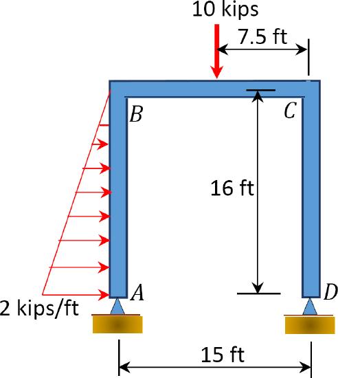
Example 11.7

Using the slope-deflection method, determine the member end moments of the frame shown in Figure 11.13a.

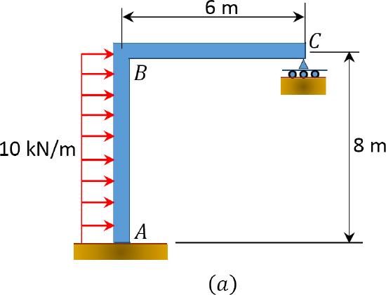
\(Fig. 11.13\). Frame.

Solution

Fixed-end moments.

The Fixed-end moments (FEM) using Table 11.1 are computed as follows:

\(\begin{array}{l}
F E M_{A B}=-\frac{w \mathrm{~L}^{2}}{12}=-\frac{10 \times 8^{2}}{12}=-53.33 \mathrm{kN} . \mathrm{m} \\
F E M_{B A}=\frac{w \mathrm{~L}^{2}}{12}=53.33 \mathrm{kN} . \mathrm{m} \\
F E M_{B C}=\mathrm{FEM}_{B C}=0
\end{array}\)

Slope-deflection equations.

As \(\theta_{A}=\psi_{B C}=0\) and \(\psi_{A B}=\frac{\Delta}{8}\) the equations for member end moments can be expressed as follows: \[\begin{aligned}
M_{A B} &=2 E K\left(2 \theta_{A}+\theta_{B}-3 \psi\right)+F E M_{A B} \\
=& 2 E K\left[\theta_{B}-3\left(\frac{-\Delta}{8}\right)\right]-53.33 \\
=& 2 E K \theta_{B}+0.75 E K \Delta-53.33
\end{aligned}\]

\[\begin{aligned}
\mathrm{M}_{\mathrm{BA}} &=2 \mathrm{EK}\left(\theta_{\mathrm{A}}+2 \theta_{\mathrm{B}}-3\left(\frac{-\Delta}{8}\right)\right)+\mathrm{FEM}_{B A} \\
=& 2 E K\left[2 \theta_{B}-3\left(\frac{-\Delta}{8}\right)\right]+53.33 \\
=& 4 E K \theta_{B}+0.75 E K \Delta+53.33
\end{aligned}\]

\[\begin{aligned}
M_{B C} &=3 E K\left(\theta_{B}-\psi\right)+\mathrm{FEM}_{B C}-\frac{\mathrm{FEM}_{C B}}{2} \\
&=3 E K \theta_{B}
\end{aligned}\]

Joint equilibrium equation.

\[\begin{array}{l}
\sum M_{B}=M_{B A}+M_{B C}=0 \\
4 E K \theta_{B}+0.75 E K \Delta+53.33+3 \mathrm{EK} \theta_{B}=0 \\
7 E K \theta_{B}+0.75 E K \Delta=-53 . .33
\end{array}\]

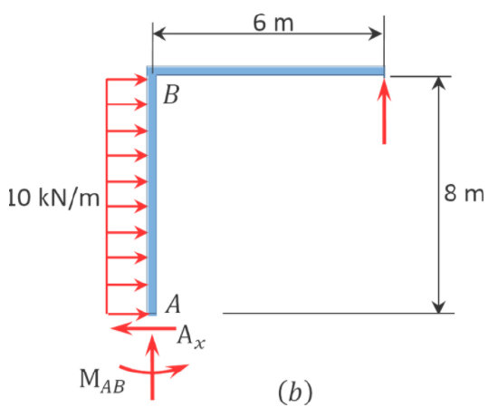
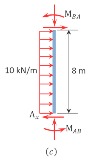
The equilibrium of the horizontal forces in Figure 11.13b suggests the following: \[\begin{array}{l}
+\rightarrow \sum F_{x}=0 \\
(10)(8)-A_{x}=0
\end{array}\]

Figure 11.13c suggests the following: \[A_{x}=\frac{M_{A B}+M_{B A}+(10)(8)(4)}{8}\]

Substituting \(A_{x}\) from equation 6 into equation 5 suggests the following: \[\begin{array}{l}
80-\frac{M_{A B}+M_{B A}+320}{8}=0 \\
640-320=M_{A B}+M_{B A}
\end{array}\]

Substituting \(M_{AB}\) and \(M_{BA}\) from equations 1 and 2 into equation 7 suggests the following: \[\begin{array}{l}
2 E K \theta_{B}+0.75 E K \Delta-53.33+4 E K \theta_{B}+0.75 E K \Delta+53.33=320 \\
6 E K \theta_{B}+1.5 E K \Delta=320
\end{array}\]

Solving equations 4 and 8 simultaneously suggests the following:

\(E K \theta_{B}=-53.33\) and \(E K \Delta=426.66\)

Final member end moments.

Putting the obtained values of \(E K \theta_{B}\) and \(E K \Delta\) into equations 1, 2, and 3 for member end moments suggests the following:

\(\begin{aligned}
\mathrm{M}_{A B}=2 \mathrm{EK} \theta_{B}+0.75 \mathrm{EK} \Delta-53.33=160 \mathrm{kN} . \mathrm{m} \\
\mathrm{M}_{B A}=4 \mathrm{EK} \theta_{B}+0.75 \mathrm{EK} \Delta+53.33=160 \mathrm{kN} . \mathrm{m} \\
\mathrm{M}_{B C}=3 \mathrm{EK} \theta_{B}=-160 \mathrm{kN} . \mathrm{m} \\
\mathrm{M}_{C B}=0
\end{aligned}\)

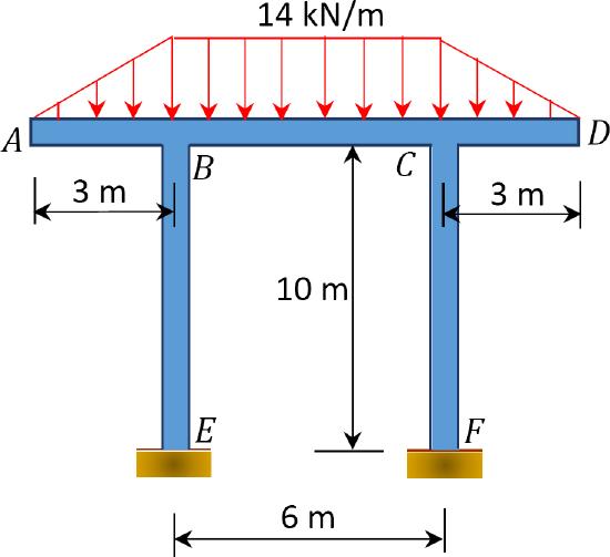
Example 11.8

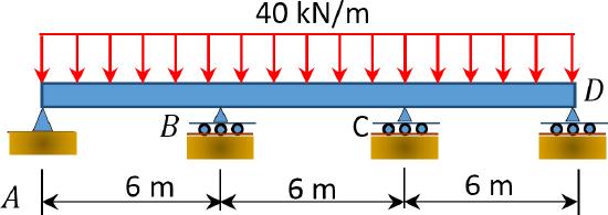
Using the slope-deflection method, determine the member end moments of the beam of the rectangular cross section shown in Figure 11.14a.

\(Fig. 11.14\). Beam.

Solution

Fixed-end moments.

The Fixed-end moments (FEM) using Table 11.1 are computed as follows:

\(\begin{array}{l}
F E M_{A B}=-\frac{P L}{8}=-\frac{40 \times 8}{8}=-40.0 \mathrm{kN} . \mathrm{m} \\
F E M_{B A}=\frac{P L}{8}=40.0 \mathrm{kN} . \mathrm{m} \\
F E M_{B C}=-\frac{P a b^{2}}{L^{2}}=-\frac{(30)(2)(4)^{2}}{6^{2}}=-26.67 \mathrm{kN} . \mathrm{m} \\
F E M_{C B}=\frac{P a^{2} b}{L^{2}}=\frac{(30)(2)^{2}(4)}{6^{2}}=13.33 \mathrm{kN} . \mathrm{m}
\end{array}\)

Slope-deflection equations.

As \(\theta_{A}=\theta_{D}=0\) and \(\psi_{A B}=\frac{\Delta}{8}\), equations for member end moments can be expressed as follows: \[\begin{aligned}
M_{A B} &=2 E K\left(2 \theta_{A}+\theta_{B}-3 \psi\right)+F E M_{A B} \\
&=2 E K\left[\theta_{B}-3\left(\frac{-\Delta}{8}\right)\right]-40 \\
&=2 E K \theta_{B}+0.75 E K \Delta-40
\end{aligned}\]

\[\begin{aligned}
M_{B A} &=2 E K\left(\theta_{A}+2 \theta_{B}-3\left(\frac{-\Delta}{8}\right)\right)+F E M_{B A} \\
&=2 E K\left[2 \theta_{B}-3\left(\frac{-\Delta}{8}\right)\right]+40 \\
&=4 E K \theta_{B}+0.75 E K \Delta+40
\end{aligned}\]

\[\begin{aligned}
M_{B C} &=2 E K\left(2 \theta_{B}+\theta_{C}-3 \psi\right)+F E M_{B C} \\
&=4 E K \theta_{B}+2 E K \theta_{C}-26.67
\end{aligned}\]

\[\begin{aligned}
\mathrm{M}_{C B}=& 2 E K\left(\theta_{B}+2 \theta_{C}\right)+F E M_{C B} \\
=& 2 E K \theta_{B}+4 E K \theta_{C}+13.33
\end{aligned}\]

\[\begin{aligned}
M_{C D} &=2 E K\left(2 \theta_{C}+\theta_{D}-3 \psi\right)+F E M_{C D} \\
&=4 E K \theta_{C}+0.75 E K \Delta
\end{aligned}\]

\[\begin{aligned}
M_{D C} &=2 E K\left(\theta_{C}+2 \theta_{D}-3 \psi\right)+F E M_{D C} \\
&=2 E K \theta_{C}+0.75 E K \Delta
\end{aligned}\]

Joint equilibrium equation. \[\begin{array}{l}
\sum M_{B}=M_{B A}+M_{B C}=0 \\
4 E K \theta_{B}+0.75 E K \Delta+40+4 E K \theta_{B}+2 E K \theta_{C}-26.67=0 \\
8 E K \theta_{B}+2 E K \theta_{C}+0.75 E K \Delta=-13.33
\end{array}\]

\[\begin{array}{l}
\sum M_{C}=M_{C B}+M_{C D}=0 \\
2 E K \theta_{B}+4 E K \theta_{C}+13.33+4 E K \theta_{C}+0.75 E K \Delta=0 \\
2 E K \theta_{B}+8 E K \theta_{C}+0.75 E K \Delta=-13.33
\end{array}\]

\[\begin{array}{l}
\sum F_{x}=0 \\
40-A_{x}-D_{x}=0
\end{array}\]

Substituting \(A_{x}=\frac{M_{A B}+M_{B A}+(40 \times 4)}{8}\) and \(D_{x}=\frac{M_{C D}+M_{D C}}{8}\) into the previous equation suggests the following: \[\begin{array}{l}
40-\frac{M_{A B}+M_{B A}+(40 \times 4)}{8}-\frac{M_{C D}+M_{D C}}{8}=0 \\
\frac{M_{A B}+M_{B A}+(40 \times 4)}{8}+\frac{M_{C D}+M_{D C}}{8}=320 \\
M_{A B}+M_{B A}+(40 \times 4)+M_{C D}+M_{D C}=320
\end{array}\]

Substituting the expressions of \(M_{AB}\), \(M_{BA}\), \(M_{CD}\) and \(M_{DC}\) from equations 1, 2, 5, and 6 into e suggests the following: \[\begin{array}{l}
2 E K \theta_{B}+0.75 E K \Delta-40+4 E K \theta_{B}+0.75 E K \Delta+40+160+4 E K \theta_{C}+0.75 E K \Delta+ \\
2 E K \theta_{C}+0.75 E K \Delta=320 \\
6 E K \theta_{B}+6 E K \theta_{C}+3 E K \Delta=160
\end{array}\]

Solving equations 7, 8, and 11 simultaneously suggests the following:

\(\begin{array}{l}
E K \theta_{B}=-7.62 \\
E K \theta_{C}=-7.62 \\
E K \Delta=83.81
\end{array}\)

Final member end moments.

Substituting the obtain values of \(E K \theta_{B}\), \(E K \theta_{C}\) and \(E K \Delta\) into member end moment equations suggests the following:

\(\begin{array}{l}
M_{A B}=2 E K \theta_{B}+0.75 E K \Delta-40=7.62 \\
M_{B A}=4 E K \theta_{B}+0.75 E K \Delta+40=72.39 \\
M_{B C}=4 E K \theta_{B}+2 E K \theta_{C}-26.67=-72.39 \\
M_{C B}=2 E K \theta_{B}+4 E K \theta_{C}+13.33=-32.39 \\
M_{C D}=4 E K \theta_{C}+0.75 E K \Delta=32.39 \\
M_{D C}=2 E K \theta_{C}+0.75 E K \Delta=47.62
\end{array}\)

\(Table 11.1\). Fixed-end moments.

Type of loading	(FEM)AB	(FEM)BA
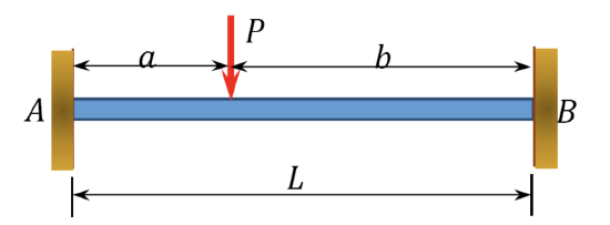	\(\frac{Pab^2}{L^2}\)	\(\frac{Pa^2b}{L^2}\)
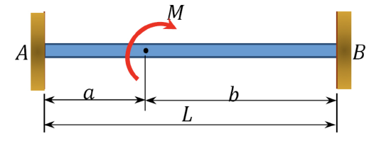	\(b(2a-b)\frac{M}{L^2}\)	\(a(2b-a)\frac{M}{L^2}\)
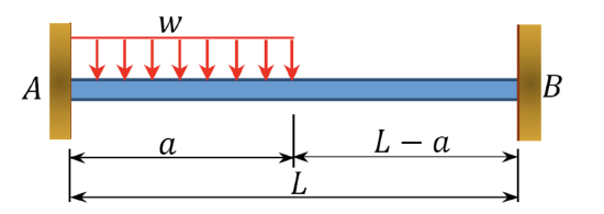	\(\frac{wL^2}{12}\left(6-8\frac{a}{L}+3\frac{a^2}{L^2}\right)\)	\(\frac{wL^2}{12}\left(4-3\frac{a}{L}\right)\)
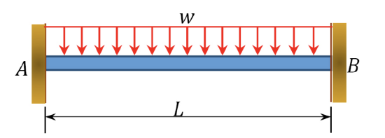	\(\frac{wL^2}{12}\)	\(\frac{wL^2}{12}\)
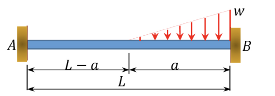	\(\frac{wa^3}{60L}\left(5-3\frac{a}{L}\right)\)	\(\frac{wa^2}{60}\left(16-10\frac{a}{L}+3\frac{a^2}{L^2}\right)\)
	\(\frac{wL^2}{30}\)	\(\frac{wL^2}{20}\)
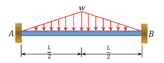	\(\frac{5wL^2}{96}\)	\(\frac{5wL^2}{96}\)

Chapter Summary

Slope-deflection method of analysis of indeterminate structures: The unknowns in the slope-deflection method of analysis are the rotations and the relative displacements. Slope-deflection equations for member-end moments and the equilibrium equation at each joint that is free to rotate are written in terms of the rotations and relative displacements, and they are solved simultaneously to determine the unknowns. When the unknown rotations and the relative displacements are determined, they are put back in member end moment equations to determine the magnitude of the moments. After determination of the end moments, the structure becomes determinate. The detailed procedures for analysis by slope-deflection method for beams and frames are presented in sections 11.5 and 11.6. In situations where there are several unknowns, analysis using this method can be very cumbersome, hence the availability of software that can perform the analysis.

Slope-deflection equations for mnd Moments:

\(\begin{array}{l}
M_{A B}=2 E K\left(2 \theta_{A}+\theta_{B}-3 \psi\right)+M_{A B}^{F} \\
M_{B A}=0=2 E K\left(\theta_{A}+2 \theta_{B}-3 \psi\right)+M_{B A}^{F}
\end{array}\)

Modified slope-deflection equation when far end is supported by a roller or pin:

\(M_{A B}=3 E K\left(\theta_{A}-\psi\right)+\left(M_{A B}^{F}-\frac{M_{B A}^{F}}{2}\right)\)

Practice Problems

11.1 Using the slope-deflection method, compute the end moment of members of the beams shown in Figure P11.1 through Figure P11.5 and draw the bending moment and shear force diagrams. \(EI =\) constant.

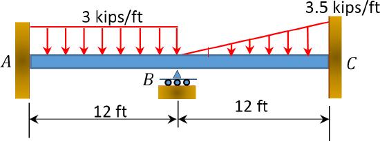
\(Fig. P11.1\). Beam.

\(Fig. P11.2\). Beam.

\(Fig. P11.3\). Beam.

\(Fig. P11.4\). Beam.

\(Fig. P11.5\). Beam.

11.2 Using the slope-deflection method, compute the end moments of members of the beams shown in Figure P11.6. Assume support \(E\) settles by 50 mm. \(E=200 \mathrm{GPa}\) and \(I=600 \times 10^{6} \mathrm{~mm}^{4}\).

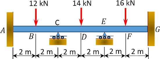
\(Fig. P11.6\). Beam.

11.3 Using the slope-deflection method, determine the end moments of the members of the non-sway frames shown in Figure P11.7 through Figure P11.10. Draw the bending moment and the shear force diagrams.

\(Fig. P11.7\). Non-sway frame.

\(Fig. P11.8\). Non – sway frame.

\(Fig. P11.9\). Non – sway frame.

\(Fig. P11.10\). Non – sway frame.

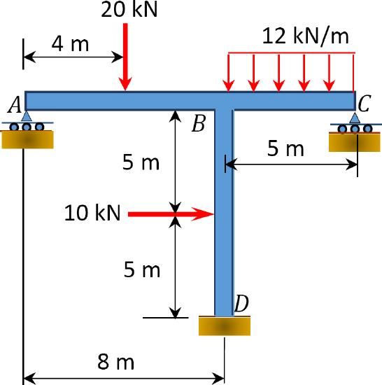
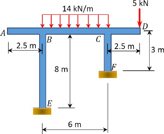
11.4 Using the slope-deflection method, determine the end moments of the members of the sway frames shown in Figure P11.11 through Figure P11.14. Draw the bending moment and the shear force diagrams.

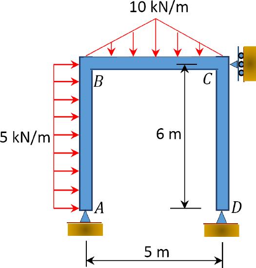
\(Fig. P11.11\). Sway frame.

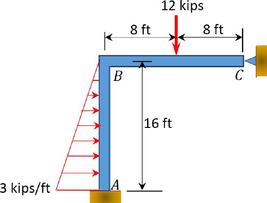
\(Fig. P11.12\). Sway frame.

\(Fig. P11.13\). Sway frame.

\(Fig. P11.14\). Sway frame.