8.2: Error Propogation

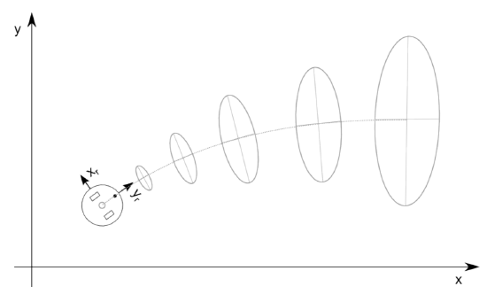
It turns out that the Gaussian Distribution is very appropriate to model prominent random processes in robotics: the robot’s position and distance measurements. A differential wheel robot that drives along a straight line, and is subject to slip, will actually increase its uncertainty the farther it drives. Initially at a known location, the expected value (or mean) of its position will be increasingly uncertain, corresponding to an increasing variance. This variance is obviously somehow related to the variance of the underlying mechanism, namely the slipping wheel and (comparably small) encoder noise. Interestingly, we will see its variance grow much faster orthogonal to the robot’s direction, as small errors in orientation have a much larger effect than small errors in longitudinal direction. This is illustrated in Figure 8.2.1.

Similarly, when estimating distance and angle to a line feature from point cloud data, the uncertainty of the random variables describing distance and angle to the line are somewhat related to the uncertainty of each point measured on the line. These relationships are formally captured by the error propagation law.

Figure \(\PageIndex{1}\): Two-dimensional Normal distribution depicting growing uncertainty as the robot moves. Albeit starting with equal uncertainty in x and y, the large effect of small errors in orientation lets the error grow faster in y-direction of the robot

The key intuition behind the error propagation law is that the variance of each component that contributes to a random variable should be weighted as a function of how strongly this component influences this random variable. Measurements that have little effect on the aggregated random variable should also have little effect on its variance and vice versa. “How strongly” something affects something else can be expressed by the ratio of how little changes of something relate to little changes in something else. This is nothing else than the partial derivative of something with respect to something else. For example, let y = f(x) be a function that maps a random variable x, e.g., a sensor reading, to a random variable y, e.g., a feature. Let the standard deviation of x be given by σ_x. We can then calculate the variance σ²_y by

\[\sigma _{y}^{2}=\left ( \frac{∂f}{∂x} \right )^{2}\sigma _{x}^{2}\]

In case y = f(x) is a multivariable function that maps n inputs to m outputs, variances become covariance matrices. A covariance matrix holds the variance of each variable along its diagonal and is zero otherwise, if the random variables are not correlated. We can then write

\[Σ^{Y}=JΣ^{X}J^{T}\]

where Σ^X and Σ^Y are the covariance matrices holding the variances of the input and output variables, respectively, and J is a mxn Jacobian matrix, which holds the partial derivatives ∂f_i/∂x_j . As J has n columns, each row contains partial derivatives with respect to x₁ to x_n.

8.2.1. Example: Line Fitting

Let’s consider an example of estimating angle α and distance r of a line from a set of points given by (ρ_i , θ_i) using Equations 7.3.4–7.3.5. We can now express the relationship of changes of a variable such as ρ_i to changes in α by

\[\frac{∂\alpha }{∂\rho _{i}}\]

Similarly, we can calculate ∂α/∂θ_i , ∂r/∂ρ_i and ∂r/∂θ_i . We can actually do this, because we have derived analytical expressions for α and r as a function of θ_i and ρ_i in Chapter 7.

We are now interested in deriving equations for calculating the variance of α and r as a function of the variances of the distance measurements. Let’s assume each distance measurement ρ_i has variance σ²_ρi and each angular measurement θ_i has variance σ²_θi . We now want to calculate σ²_α as the weighted sum of σ²_ρi and σ²_θi , each weighted by its influence on α. More generally, if we have I input variables X_i and K output variables Y_k, the covariance matrix of the output variables σ_Y can be expressed as σ²_Y = ∂f²/∂X σ²_X where σ_X is the covariance matrix of input variables and J is a Jacobian matrix of a function f that calculates Y from X and has the form

\[J=\begin{bmatrix}
\frac{∂f_{1}}{∂X_{1}} & \cdots &\frac{∂f_{1}}{∂X_{1}} \\
\vdots & \cdots &\vdots \\
\frac{∂f_{K}}{∂X_{1}} & \cdots & \frac{∂f_{K}}{∂X_{1}}
\end{bmatrix}\]

In the line fitting example F_X would contain the partial derivatives of α with respect to all ρ_i (i-entries) followed by the partial derivates of α with respect to all θ_i in the first row. In the second row, F_X would hold the partial derivates of r with respect to ρ_i followed by the partial derivates of r with respect to θ_i . As there are two output variables, α and r, and 2I input variables (each measurement consists of an angle and distance), F_X is a 2 x (2I) matrix.

The result is therefore a 2x2 covariance matrix that holds the variances of α and r on its diagonal.

8.2.2. Example: Odometry

Whereas the line fitting example demonstrated a many-toone mapping, odometry requires to calculate the variance that results from multiple sequential measurements. Error propagation allows us here to not only express the robot’s position, but also the variance of this estimate. Our “laundry list” for this task looks as follows:

1. What are the input variables and what are the output variables?
2. What are the functions that calculate output from input?
3. What is the variance of the input variables?

As usual, we describe the robot’s position by a tuple (x, y, θ). These are the three output variables. We can measure the distance each wheel travels ∆s_r and ∆s_l based on the encoder ticks and the known wheel radius. These are the two input variables. We can now calculate the change in the robot’s position by calculating

\[\Delta x=\Delta scos(\theta +\Delta \theta /2)\]

\[\Delta y=\Delta ssin(\theta +\Delta \theta /2)\]

\[\Delta \theta =\frac{\Delta s_{r}-\Delta s_{l}}{b}\]

with

\[\Delta s =\frac{\Delta s_{r}+\Delta s_{l}}{2}\]

The new robot’s position is then given by

\[f(x,y,\theta ,\Delta s_{r},\Delta s_{l})=\left [ x,y,\theta \right ]^{T}+\begin{bmatrix}
\Delta x & \Delta y & \Delta \theta
\end{bmatrix}^{T}\]

We thus have now a function that relates our measurements to our output variables. What makes things complicated here is that the output variables are a function of their previous values. Therefore, their variance does not only depend on the variance of the input variables, but also on the previous variance of the output variables. We therefore need to write

\[Σ_{p'}=∇_{p}fΣ_{p}∇_{p}f^{T}+∇_{\Delta_{r,l}}fΣ_{\Delta }∇_{\Delta_{r,l}}f^{T}\]

The first term is the error propagation from a position p = [x, y, θ] to a new position p 0 . For this we need to calculate the partial derivatives of f with respect to x, y and θ. This is a 3x3 matrix

\[∇_{p}f=\begin{bmatrix}
\frac{∂f}{∂x} & \frac{∂f}{∂y} & \frac{∂f}{∂\theta }
\end{bmatrix}=\begin{bmatrix}
1 & 0 & -\Delta ssin(\theta +\Delta \theta /2)\\
0& 1 & \Delta scos(\theta +\Delta \theta /2)\\
0& 0 & 1
\end{bmatrix}\]

The second term is the error propagation of the actual wheel slip. This requires calculating the partial derivatives of f with respect to ∆s_r and ∆s_l , which is a 3x2 matrix. The first column contains the partial derivatives of x, y, θ with respect to ∆s_r. The second column contains the partial derivatives of x, y, θ with respect to ∆s_l :

\[∇_{\Delta _{r,l}}f=\begin{bmatrix}
\frac{1}{2}\cos(\theta +\frac{\Delta \theta /2}{b})-\frac{\Delta s}{2b} \sin(\theta +\frac{\Delta \theta }{b})& \frac{1}{2}\cos(\theta +\frac{\Delta \theta /2}{b})-\frac{\Delta s}{2b} \sin(\theta +\frac{\Delta \theta }{b})\\
\frac{1}{2}\sin(\theta +\frac{\Delta \theta /2}{b})+\frac{\Delta s}{2b} \sin(\theta +\frac{\Delta \theta }{b})& \frac{1}{2}\sin(\theta +\frac{\Delta \theta /2}{b})+\frac{\Delta s}{2b} \sin(\theta +\frac{\Delta \theta }{b})\\
\frac{1}{2}& -\frac{1}{2}
\end{bmatrix}\]

Finally, we need to define the covariance matrix for the measurement noise. As the error is proportional to the distance traveled, we can define Σ_∆ by

\[Σ_{\Delta }=\begin{bmatrix}
k_{r}\left | \Delta s_{r} \right | & 0\\
0 & k_{l}\left | \Delta s_{l} \right |
\end{bmatrix}\]

Here _kr and k_l are constants that need to be found experimentally and | · | indicating the absolute value of the distance traveled. We also assume that the error of the two wheels is independent, which is expressed by the zeros in the matrix.

We now have all ingredients for Equation 8.2.10, allowing us to calculate the covariance matrix of the robot’s pose much like shown in Figure 8.2.1.