9.2: Markov Localization

Calculating the probability to be at a certain location given the likelihood of certain observations is nothing else as a conditional probability. There is a formal way to describe such situations: Bayes’ Rule (Section C.2):

\[P(A|B)=\frac{P(A)P(B|A)}{P(B)}\]

9.2.1. Perception Update

How does this map into a Localization framework? Let’s assume, event A is equivalent to be at a specific location loc. Lets also assume that event B corresponds to the event to see a particular feature feat. We can now rewrite Bayes’ rule to

\[P(loc|feat)=\frac{P(loc)P(feat|loc)}{P(feat)}\]

Rephrasing Bayes’ rule in this way, we can calculate the probability to be at location loc, given that we see feature feat. This is known as Perception Update. For example, loc could correspond to door 1, 2 or 3, and feat could be the event of sensing a door. What do we need to know to make use of this equation?

1. We need to know the prior probability to be at location loc P(loc)
2. We need to know the probability to see the feature at this location P(feat|loc)
3. We need the probability to encounter the feature feat P(feat)

Figure \(\PageIndex{1}\): A robot localizing itself using a “door detector” in a known map. Top: Upon encountering a door, the robot can be in front of any of the three doors. Middle: When driving to the right, the Gaussian distributions representing its location also shift to the right and widen, representing growing uncertainty. Bottom: After detecting the second door, the robot can discard hypotheses that are not in front of the door and gains certainty on its location.

Let’s start with (3), which might be the most confusing part of information we need to collect. The answer is simple, no matter what P(feat) is, it will cancel out as the probability to be at any of the possible locations has to sum up to 1. (A simpler, although less accurate, explanation would be that the probability to sense a feature is constant and therefore does not matter.)

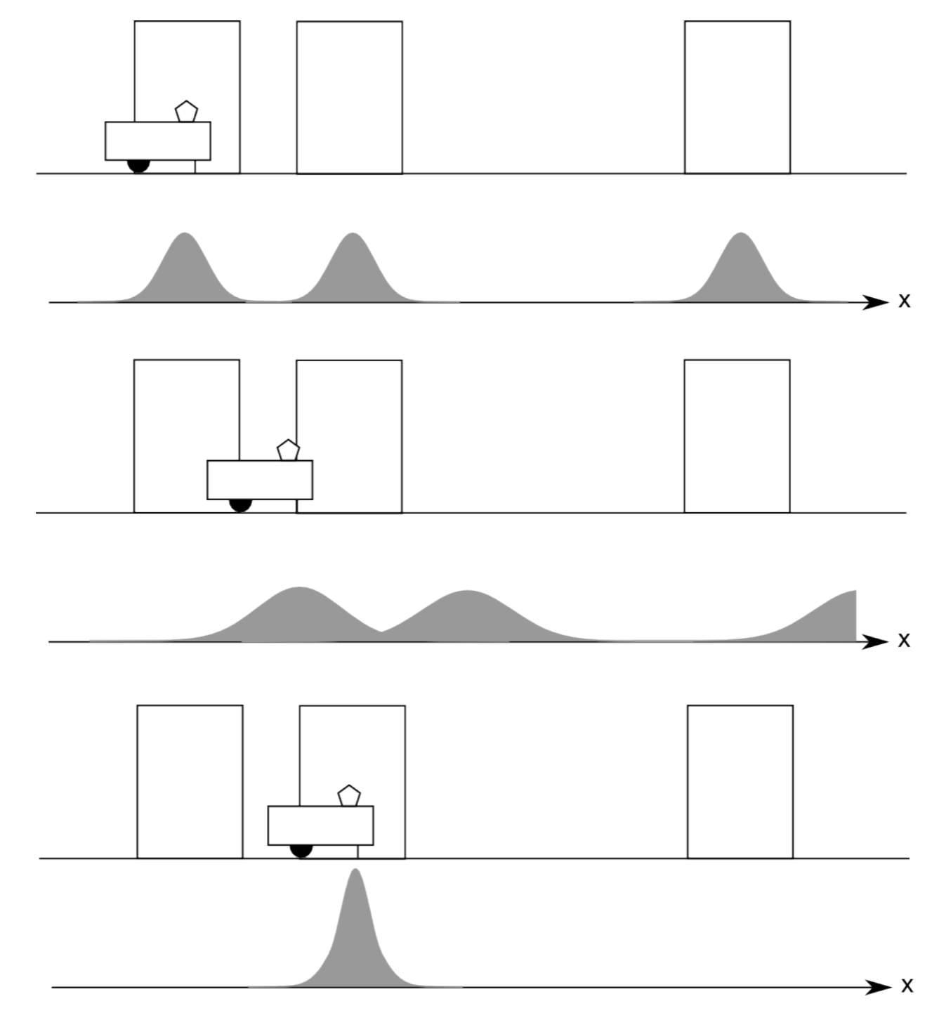
The prior probability to be at location loc, P(loc), is called the belief model. In the case of the 3-door example, it is the value of the Gaussian distribution underneath the door corresponding to loc.

Finally, we need to know the probability to see the feature feat at location loc P(feat|loc). If your sensor were perfect, this probability is simply 1 if the feature exists at this location, or 0 if the feature cannot be observed at this location. If your sensor is not perfect, P(feat|loc) corresponds to the likelihood for the sensor to see the feature if it exists.

The final missing piece is how to best represent possible locations. In the graphical example in Figure 9.2.1 we assumed Gaussian distributions for each possible location. Alternatively, we can also discretize the world into a grid and calculate the likelihood of the robot to be in any of its cells. In our 3-door world, it might make sense to choose grid cells that have just the width of a door.

9.2.2. Action Update

One of the assumptions in the above thought experiment was that we know with certainty that the robot moved right. We will now more formally study how to treat uncertainty from motion. Recall that odometry input is just another sensor that we assume to have a Gaussian distribution; if our odometer tells us that the robot traveled a meter, it could have traveled a little less or a little more, with decreasing likelihood. We can therefore calculate the posterior probability of the robot moving from a position loc' to loc given its odometer input odo:

\[P(loc'->loc|odo)=P(loc'->loc)P(odo|loc'->loc)/P(odo)\]

This is again Bayes’ rule. The unconditional probability P(loc'− > loc) is the prior probability for the robot to have been at location loc' . The term P(odo|loc'− > loc) corresponds to the probability to get odometer reading odo after traveling from a position loc' to loc. If getting a reading of the amount odo is reasonable for the distance from loc' to loc this probability is high. If it is unreasonable, for example if the distance is larger than what is physically possible, this probability should be very low.

As the robot’s location is uncertain, the real challenge is now that the robot could have potentially been everywhere to start with. We therefore have to calculate the posterior probability P(loc|odo) for all possible positions loc' . This can be accomplished by summing over all possible locations:

\[P(loc|odo)=\sum_{loc'}^{}P(loc'->loc)P(odo|loc'->loc)\]

In other words, the law of total probability requires us to consider all possible locations the robot could have ever been at. This step is known as Action Update. In practice we don’t need to calculate this for all possible locations, but only those that are technically feasible given the maximum speed of the robot. We note also that the sum notation technically corresponds to a convolution (Section C.3) of the probability distribution of the robot’s location in the environment with the robot’s odometry error probability distribution.

9.2.3. Summary and Examples

We have now learned two methods to update the belief distribution of where the robot could be in the environment. First, a robot can use external landmarks to update its position. This is known as perception update and relies on exterioception. Second, a robot can observe its internal sensors. This is known as action update and relies on proprioception. The combination of action and perception updates is known as Markov Localization. You can think about the action update to increase the uncertainty of the robot’s position and the perception update to shrink it. (You can also think about the action update as a discrete version of the error propagation model.) Also here we are using the robotics kinematic model and the noise model of your odometer to calculate P(odo|loc'− > loc).

Figure \(\PageIndex{2}\): An office environment consisting of two rooms connected by a hallway. A topological map is super-imposed.

Example \(\PageIndex{1}\): Topological Map

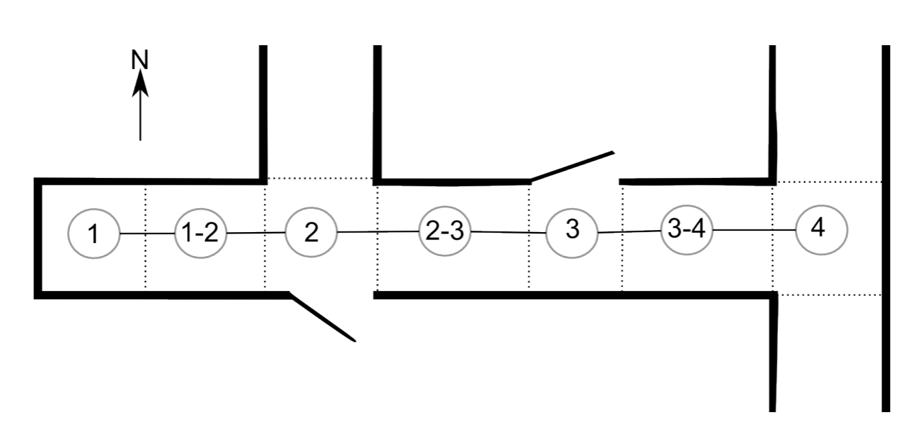
This example describes one of the first successful real robot systems that employed Markov Localization in an office environment. The experiment is described in more detail in a 1995 article of AI Magazine(?). The office environment consisted of two rooms and a corridor that can be modeled by a topological map (Figure 9.2.2). In a topological map, areas that the robot can be in are modeled as vertices, and navigable connections between them are modeled as edges of a graph. The location of the robot can now be represented as a probability distribution over the vertices of this graph.

The robot has the following sensing abilities:

• It can detect a closed door to its left or right.
• It can detect an open door to its left or right.
• It can detect whether it is an open hallway.

Table	Wall	Closed Dr	Open Dr	Open Hwy	Foyer
Nothing Detected	70%	40%	5%	0.1%	30%
Closed Door Detected	30%	60%	0%	0%	5%
Open Door Detected	0%	0%	90%	10%	15%
Open Hallway Detected	0%	0%	0.1%	90%	50%

Table \(\PageIndex{1}\): Conditional probabilities of the Dervish robot detecting certain features in the Stanford laboratory.

Unfortunately, the robot’s sensors are not at all reliable. The researchers have experimentally found the probabilities to obtain a certain sensor response for specific physical positions using their robot in their environment. These values are provided in Table 9.2.1.

For example, the success rate to detect a closed door is only 60%, whereas a foyer looks like an open door in 15% of the trials. This data corresponds to the conditional probability to detect a certain feature given a certain location.

Consider now the following initial belief state distribution: p(1 − 2) = 0.8 and p(2 − 3) = 0.2. Here, 1 − 2 etc. refers to the position on the topological map in Figure 9.2.2. You know that the robot faces east with certainty. The robot now drives for a while until it reports “open hallway on its left and open door on its right”. This actually corresponds to location 2, but the robot can in fact be anywhere. For example there is a 10% chance that the open door is in fact an open hallway, i.e. the robot is really at position 4. How can we calculate the new probability distribution of the robot’s location? Here are the possible trajectories that could happen:

The robot could move from 2−3 to 3, 3−4 and finally 4. We have chosen this sequence as the probability to detect an open door on its right is zero for 3 and 3 − 4, which leaves position 4 as the only option if the robot has started at 2 − 3. In order for this hypothesis to be true, the following events need to have happened, their probabilities are given in parentheses:

1. The robot must have started at 2 − 3 (20%)
2. Not have seen the open door at the left of 3 (5%) and not have seen the wall at the right (70%)
3. Not have seen the wall to its left (70%) and not have seen the wall to its right at node 3 − 4 (70%)
4. Correctly identify the open hallway to its left (90%) and mistake the open hallway to its right for an open door (10%)

Together, the likelihood that the robot got from position 2 − 3 to position 4 is therefore given by 0.2 × 0.05 × 0.7 × 0.7 × 0.7 × 0.9 × 0.1 = 0.03%, that is very unlikely.

The robot could also move from 1 − 2 to 2, 2 − 3, 3, 3 − 4 or 4. We can evaluate these hypotheses in a similar way:

• The chance that it correctly detects the open hallway and door at position 2 is 0.9 × 0.9, so the chance to be at position 2, having started at 1−2, is 0.8×0.9×0.9 = 64%.
• The robot cannot have ended up at position 2 − 3, 3, and 3 − 4 because the chance of seeing an open door instead of a wall on the right side is zero in all these cases.
• In order to reach position 4, the robot must have started at 1−2 has a chance of 0.8. The robot must not have seen the hallway on its left and the open door to its right when passing position 2. The probability for this is 0.001×0.05. The robot must then have detected nothing at 2−3 (0.7× 0.7), nothing at 3 (0.05×0.7), nothing at 3−4 (0.7×0.7), and finally mistaken the hallway on its right for an open door at position 4 (0.9 × 0.1). Multiplied together, this outcome is very unlikely.

Given this information, we can now calculate the posterior probability to be at a certain location on the topological map by adding up the probabilities for every possible path to get there.

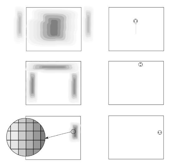
Example \(\PageIndex{2}\): Grid-Based Markov Localization

Instead of using a coarse topological map, we can also model the environment as a fine-grained grid. Each cell is marked with a probability corresponding to the likelihood of the robot being at this exact location (Figure 9.2.3). We assume that the robot is able to detect walls with some certainty. The images in the right column show the actual location of the robot. Initially, the robot does not see a wall and therefore could be almost anywhere. The robot now moves northwards. The action update now propagates the probability of the robot being somewhere upwards. As soon as the robot encounters the wall, the perception update bumps up the likelihood to be anywhere near a wall. As there is some uncertainty associated with the wall detector, the robot cannot only be directly at the wall, but anywhere — with decreasing probability — close by. As the action update involved continuous motion to the north, the likelihood to be close to the south wall is almost zero. The robot then performs a right turn and travels along the wall in clockwise direction. As soon as it hits the east wall, it is almost certain about its position, which then again decreases.

Figure \(\PageIndex{3}\): Markov localization on a grid. The left column shows the likelihood to be in a specific cell as grey value (dark colors correspond to high likelihoods). The right column shows the actual robot location. Arrows indicate previous motion. Initially, the position of the robot is unknown, but recorded upwards motion makes positions at the top of the map more likely. After the robot has encountered a wall, positions away from walls become unlikely. After rightwards and down motions, the possible positions have shrunk to a small area.