15.1: Random Variables and Probability Distributions

Random variables can describe either discrete variables, such as the result from throwing a dice, or continuous variables such as measuring a distance. In order to learn about the likelihood that a random variable has a certain outcome, we can repeat the experiment many times and record the resulting random variates, that is the actual values of the random variable, and the number of times they occurred. For a perfectly cubic dice we will see that the random variable can hold natural numbers from 1 to 6, that have the same likelihood of 1/6.

The function that describes the probability of a random variable to take certain values is called a probability distribution. As the likelihood of all possible random variates in the dice experiment is the same, the dice follows what we call a uniform distribution. More accurately, as the outcomes of rolling a dice are discrete numbers, it is actually a discrete uniform distribution. Most random variables are not uniformly distributed, but some variates are more likely than others. For example, when considering a random variable that describes the sum of two simultaneously thrown dice, we can see that the distribution is anything but uniform:

\[2:1+1\rightarrow \frac{1}{6}\frac{1}{6}\\
3:1+2, 2+1\rightarrow 2\frac{1}{6}\frac{1}{6}\\
4 : 1 + 3, 2 + 2, 3 + 1\rightarrow 3\frac{1}{6}\frac{1}{6}\\
5 : 1 + 4, 2 + 3, 3 + 2, 4 + 1\rightarrow 4\frac{1}{6}\frac{1}{6}\\
6 : 1 + 5, 2 + 4, 3 + 3, 4 + 2, 5 + 1\rightarrow 5\frac{1}{6}\frac{1}{6}\\
7 : 1 + 6, 2 + 5, 3 + 4, 4 + 3, 5 + 2, 6 + 1\rightarrow 6\frac{1}{6}\frac{1}{6}\\
8 : 1 + 5, 2 + 4, 3 + 3, 4 + 2, 5 + 1\rightarrow 5\frac{1}{6}\frac{1}{6}\\
9 : 1 + 4, 2 + 3, 3 + 2, 4 + 1\rightarrow 4\frac{1}{6}\frac{1}{6}\\
10 : 1 + 3, 2 + 2, 3 + 1\rightarrow 3\frac{1}{6}\frac{1}{6}\\
11:1+2, 2+1\rightarrow 2\frac{1}{6}\frac{1}{6}\\
12:1+1\rightarrow \frac{1}{6}\frac{1}{6}\\\nonumber\]

As one can see, there are many more possibilities to sum up to a 7 than there are to a 3, e.g. While it is possible to store probability distributions such as this one as a look-up table to predict the outcome of an experiment (or that of a measurement), we can also calculate the sum of two random processes analytically (Section C.3).

15.1.1. The Normal Distribution

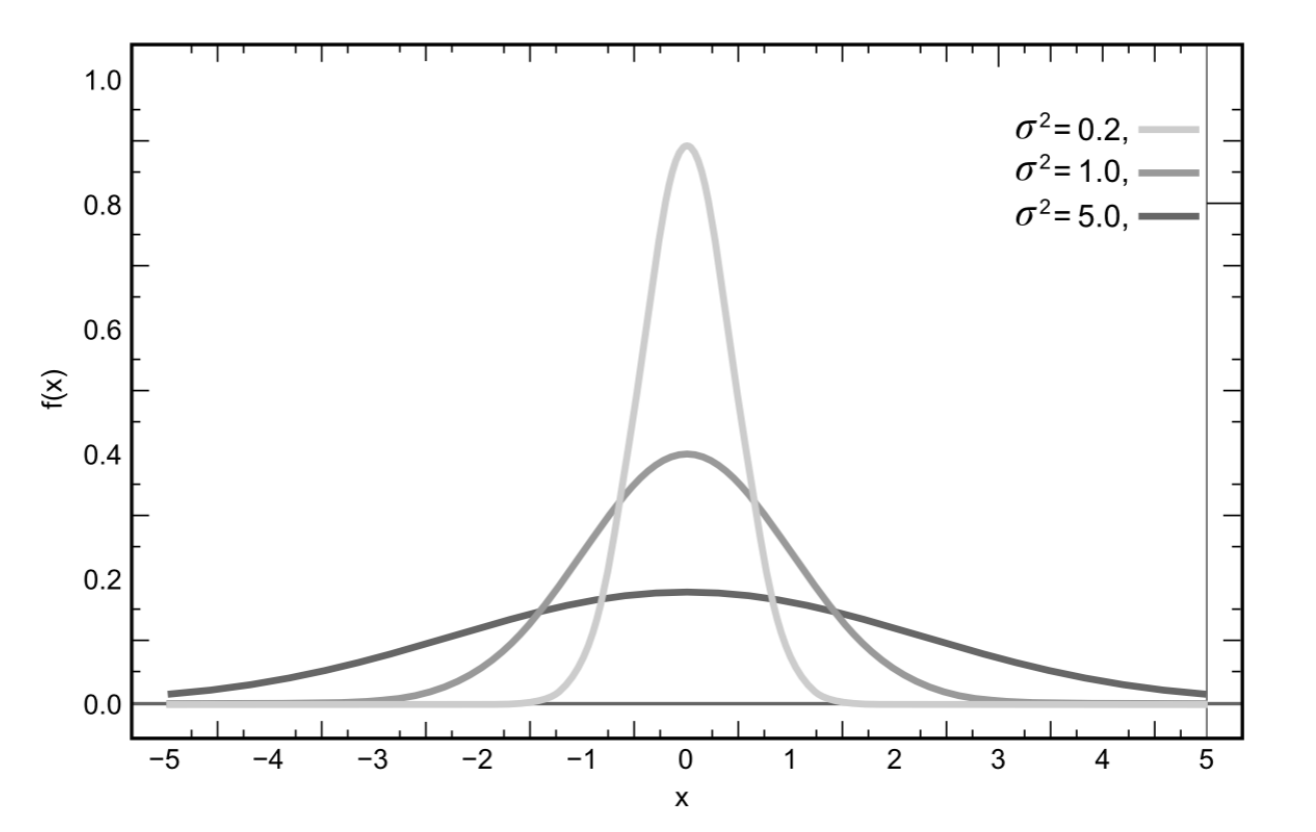
One of the most prominent distribution is the Gaussian or Normal Distribution. The Normal distribution is characterized by a mean and a variance. Here, the mean corresponds to the average value of a random variable (or the peak of the distribution) and the variance is a measure of how broadly variates are spread around the mean (or the width of the distribution). The Normal distribution is defined by the following function

\[f(x)=\frac{1}{\sqrt{2\pi \sigma ^{2}}}e^{-\frac{(x-\mu)^{2} }{2\sigma ^{2}}}\]

where µ is the mean and σ² the variance. (σ on its own is known as the standard deviation.) Then, f(x) is the probability for a random variable X to have value x. The mean is calculated by

\[\mu =\int_{-\infty }^{\infty }xf(x)dx\]

or in other words, each possible value x is weighted by its likelihood and added up.

Figure \(\PageIndex{1}\): Normal distribution for different variances and µ = 0.

The variance is calculated by

\[\sigma ^{2}=\int_{-\infty }^{\infty }(x-\mu )^{2}f(x)dx\]

or in other words, we calculate the deviation of each random variable from the mean, square it, and weigh it by its likelihood. Although it is tantalizing to perform this calculation also for the double dice experiment, the resulting value is questionable, as the double dice experiment does not follow a Normal distribution. We know this, because we actually enumerated all possible outcomes. For other experiments, such as grades in the classes you are taking, we don’t know what the real distribution is.

15.1.2. Normal Distribution in Two Dimensions

The Normal Distribution is not limited to random processes with only one random variable. For example, the X/Y position of a robot in the plane is a random process with two dimensions. In case of a multi-variate distribution with k dimensions, the random variable X is a k-dimensional vector of random variables, µ is a k-dimensional vector of means, and σ gets replaced with Σ, a k-by-k dimensional covariance matrix (a matrix that carries the variances of each random variable in its diagonal).