17.1: An Introduction to Autonomous Mobile Robots

This describes a possible one semester curriculum, which takes the students from the kinematics of a differential-wheel platform to SLAM. This curriculum is involved and requires a firm background in trigonometry, probability theory and linear algebra. This might be too ambitious for third-year Computer Science students, but fares well with Aerospace and Electrical Engineering students, who often have a stronger, and more applied, mathematical background. This curriculum is therefore also well suited as “advanced class”, e.g. in the fourth year of a CS curriculum.

17.1.1. Overview

The curriculum is motivated by a maze-solving competition that is described in Section 1.3. Solving the game can be accomplished using a variety of algorithms ranging from wall following (which requires simple proportional control) to Depth-first Search on the maze to full SLAM. Here, the rules are designed such that creating a map of the environment leads to a competitive advantage on the long run.

17.1.2. Materials

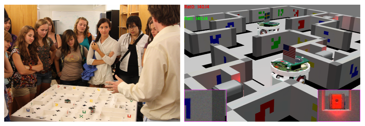
The competition can be easily re-created using card board or LEGO bricks and any miniature, differential wheel platform that is equipped with a camera to recognize simple markers in the environment (which serve as landmarks for SLAM). The setup can also easily be simulated in a physics-based simulation environment, which allows scaling this curriculum to a large number of participants. The setup used at CU Boulder using the e-Puck robot and the Webots simulator is shown in Figure 17.1.1.

Figure \(\PageIndex{1}\): The “Ratslife” maze competition created from LEGO bricks and e-Puck robots (left). The same environment simulated in Webots.

17.1.3. Content

After introducing the field and the curriculum using Chapter 1 “Introduction”, another week can be spent on basic concepts from Chapter 2 “Locomotion and Manipulation”, which includes concepts like “Static and Dynamic Stability” and “Degreesof-Freedom”. The lab portions of the class can at this time be used to introduce the software and hardware used in the competition. For example, students can experiment with the programming environment of the real robot or setup a simple world in the simulator themselves.

The lecture can then take up pace with Chapter 3. Here, the topics “Coordinate Systems and Frames of Reference”, “Forward Kinematics of a Differential Wheels Robot”, and “Inverse Kinematics of Mobile Robots” are on the critical path, whereas other sections in Chapter 3 are optional. It is worth mentioning that the forward kinematics of non-holonomic platforms, and in particular the motivation for considering their treatment in velocity rather than position space, are not straightforward and therefore at least some treatment of arm kinematics is recommended. These concepts can easily be turned into practical experience during the lab session.

The ability to implement point-to-point motions in configuration space thanks to knowledge of inverse kinematics, directly lends itself to “Map representations” and “Path Planning” treated in Chapter 4. For the purpose of maze solving, simple algorithms like Dijkstra’s and A* are sufficient, and sampling-based approaches can be skipped. Implementing a path-planning algorithm both in simulation and on the real robot will provide first-hand experience of uncertainty.

The lecture can then proceed to “Sensors” (Chapter 5), which should be used to motivate uncertainty using concepts like accuracy and precision. These concepts can be formalized using materials in Chapter C “Statistics”, and quantified during lab. Here, having students record the histogram of sensor noise distributions is a valuable exercise.

Chapters 6 and 7, which are on “Vision” and “Feature extraction”, do not need to extend further than needed to understand and implement simple algorithms for detecting the unique features in the maze environment. In practice, these can usually be detected using basic convolution-based filters from Chapter 6, and simple post-processing, introducing the notion of a “feature”, but without reviewing more complex image feature detectors. The lab portion of the class should be aimed at identifying markers in the environment, and can be scaffolded as much as necessary.

In-depth experimentation with sensors, including vision, serves as a foundation for a more formal treatment of uncertainty in Chapter 8 “Uncertainty and Error Propagation”. Depending on whether the “Example: Line Fitting” example has been treated in Chapter 7, it can be used here to demonstrate error propagation from sensor uncertainty, and should be simplified otherwise. In lab, students can actually measure the distribution of robot position over hundreds of individual trials (this is an exercise that can be done collectively if enough hardware is available), and verify their math using these observations. Alternatively, code to perform these experiments can be provided, giving the students more time to catching up.

The localization problem introduced in Chapter 9 is best introduced using Markov localization, from which more advanced concepts such as the particle filter and the Kalman filter can be derived. Performing these experiments in the lab is involved, and is best done in simulation, which allows neat ways to visualize the probability distributions changing.

The lecture can be concluded with “EKF SLAM” in Chapter 11. Actually implementing EKF SLAM is beyond the scope of an undergraduate robotics class and is achieved only by very few students who go beyond the call of duty. Instead, students should be able to experience the workings of the algorithm in simulation, e.g., using one of the many available Matlab implementations, or scaffolded in the experimental platform by the instructor.

The lab portion of the class can be concluded by a competition in which student teams compete against each other. In practice, winning teams differentiate themselves by the most rigorous implementation, often using one of the less complex algorithms, e.g., wall following or simple exploration. Here, it is up to the instructor incentivizing a desired approach.

Depending on the pace of the class in lecture as well as the time that the instructor wishes to reserve for implementation of the final project, lectures can be offset by debates, as described in Section 17.3.