8.2: One-Dimensional Continuous Motion

Imagine we have a particle that is moving along a single axis. At any given point in time, this particle will have a position, which we can quantify with a single number which we will call \(x\). This value will measure the distance from some set origin point to the position of the particle. If the particle is moving over time, we will need a function to describe the position over time \(x(t)\). This is an equation where if we plug a value for \(t\), it will give us the position at that time.

Figure \(\PageIndex{1}\): The position of a particle in one dimension can be described with a single number. If the position is changing over time, we will use the function \(x(t)\) to describe the position at any given point in time.

The velocity of the particle is then the rate of change of the position over time. If the particle is not moving, then position is not changing over time and the velocity is zero. If the particle is moving, we will first need to find the equation for position \(x(t)\), and then take the derivative of the position equation to find the velocity equation \(v(t)\). Velocity differs from speed in that the velocity has a direction (either positive or negative for now) while the speed is simply the magnitude of the velocity (always a positive number).

Next up is the acceleration, which is the rate of change of the velocity over time. If the velocity is not changing, the acceleration will be zero. If the velocity does change over time, then we will need to take the derivative of the velocity equation \(v(t)\) to find the acceleration equation \(a(t)\). The acceleration is then also the double derivative of the position equation over time. Like the velocity, the acceleration has both a magnitude and a direction.

To simplify the notation, we often use a dot on top of the variable to indicate a time derivative. This makes the velocity (the derivative of \(x\)) \(\dot{x}\) and the acceleration (the derivative of the derivative of \(x\)) \(\ddot{x}\). These relationships and their shorthand notations are all shown below.

\begin{align} \text{Position:} \quad &\, x(t) \\ \text{Velocity:} \quad &\, v(t) = \frac{dx}{dt} = \dot{x} \\ \text{Acceleration:} \quad &\, a(t) = \frac{dv}{dt} = \frac{d^2 x}{dt^2} = \ddot{x} \end{align}

If we instead start with the equation for acceleration, we can take the integral of that equation \(a(t)\) to find the equation for velocity, \(v(t)\). But unlike the derivatives, we will have an extra step in this process because whenever we integrate we wind up with a constant of integration (which we will usually call \(C\)). When we integrate the acceleration equation to find the velocity equation, this constant will be the initial velocity (the velocity at time = 0).

Next we can take the integral of the velocity equation \(v(t)\) to find the position equation \(x(t)\). With this integration we will again wind up with a constant of integration, which in this case will be the initial position (the position at time = 0). These relationships are shown below.

\begin{align} \text{Acceleration:} \quad &\, a(t) \\ \text{Velocity:} \quad &\, v(t) = \int a(t) \\ \text{Position:} \quad &\, x(t) = \int v(t) = \iint a(t) \end{align}

Constant Acceleration Systems:

In cases where we have a constant acceleration (often due to a constant force), we can start with a constant value for \(a(t) = a\), and work out the integrals from there. Along the way we will add the initial velocity and the initial position as the constants of integration to wind up with the formulas below.

\begin{align} \text{Acceleration:} \quad &\, a(t) = a \\ \text{Velocity:} \quad &\, v(t) = at + v_0 \\ \text{Position:} \quad &\, x(t) = \frac{1}{2} a t^2 + v_0 t + x_0 \end{align}

If we take the equations for the position and the velocity from above, then solve both of them for \(t\) and set those equations equal to one another, we can actually wind up with another equation that directly relates position, velocity, and acceleration without needing to know the time.

\[ v^2 - v_0^2 = 2a(x - x_0) \]

It is important to remember that these equations are only valid when the acceleration is constant. When that is not the case, you will need to use calculus to find the derivatives or integrals based on the equations for position, velocity, and acceleration that you do know.

Video lecture covering this section, delivered by Dr. Jacob Moore. YouTube source: https://youtu.be/uemxYyLN3-U.

Example \(\PageIndex{1}\)

You are in a van that steadily accelerates from 20 m/s to 35 m/s over the course of 10 seconds. What is your rate of acceleration?

Figure \(\PageIndex{2}\): A black van accelerating at a constant rate.

Solution

Video \(\PageIndex{2}\): Worked solution to example problem \(\PageIndex{1}\), provided by Dr. Majid Chatsaz. YouTube source: https://youtu.be/19qGXfNkWcQ.

Example \(\PageIndex{2}\)

You are in a van that steadily accelerates from 20 m/s to 35 m/s over the course of 10 seconds. How many meters did you travel in those ten seconds?

Figure \(\PageIndex{3}\): A black van accelerating at a constant rate.

Solution

Video \(\PageIndex{3}\): Worked solution to Example \(\PageIndex{2}\), provided by Dr. Majid Chatsaz. YouTube source: https://youtu.be/hjyUHnw8FSI.

Example \(\PageIndex{3}\)

In a rocket sled deceleration experiment, a manned sled is decelerated from a speed of 200 mph (89.4 m/s) to a stop at a constant rate of 18 G's (176.6 m/s²). How long does it take for the sled to stop? How far does the sled travel while decelerating?

Figure \(\PageIndex{4}\): A rocket sled decelerating at a constant rate.

Solution

Video \(\PageIndex{4}\): Worked solution to Example \(\PageIndex{3}\), provided by Dr. Majid Chatsaz. YouTube source: https://youtu.be/bXzcdpaxB_c.

Example \(\PageIndex{4}\)

A metallic particle is accelerated in a magnetic field such that its velocity over time is defined by the function \(v(t) = 4t^2 - 12\), where time is in seconds and velocity is in meters per second. If we assume that the particle has an initial position of zero \((x_0 = 0)\), what are the equations that describe the acceleration and position over time?

Figure \(\PageIndex{5}\): A particle accelerator.

Solution

Video \(\PageIndex{5}\): Worked solution to Example \(\PageIndex{4}\), provided by Dr. Majid Chatsaz. YouTube source: https://youtu.be/AWhLmMhKygg.

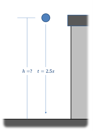
Question 4:

An object is released from rest at the top of a tall building of unknown height. Using a precision stopwatch, you note that it takes 2.5 seconds for the object to hit the ground. Assuming the standard rate of acceleration of 32.2 ft/s² and negligible air resistance, what is the estimated height of the building in feet?

Solution: