11.3: The Impulse-Momentum Principle for Particles

As stated in the previous section, the Impulse-Momentum Theorem can be boiled down to the idea that the impulse exerted on a body over a given time will be equal to the change in that body's momentum. The impulse is usually denoted by the variable J and the momentum is a body's mass times it's velocity. Impulses and velocities are both vector quantities, giving us the basic equation below.

\[\vec{J}=m \vec{v}_f-m \vec{v}_i\]

Solving Impulse Momentum Problems:

As with many mechanics problems, the best place to start an impulse momentum problem is with a diagram. Similar to the work and energy diagrams, the point is to create a diagram showing the initial state, the final state, and the forces in between causing the change. In your diagram you should show any known masses, any known velocities (magnitude and direction), any forces causing an impulse, and the time the force is exerted for (or the force function).

The impulse momentum diagram should show the initial and final states and any forces causing an impulse in between.

After creating the impulse and momentum diagram, the next step is to plug values into the equations. Put any known masses, velocities, forces, and times into the equation. If you are working in a single dimension, you will have a single equation, but you have forces and velocities in two dimensions we can break the single vector equation down into two scalar components to solve. In this case, we simply need to break all forces and velocities into x and y components.

\[\begin{array}
J_x=m v_{f x}-m v_{i x} \\
J_y=m v_{f y}-m v_{i y}
\end{array}\]

Finally, the last step will be to use algebra to solve for unknown values. With a single equation we can solve for an single unknown, with two equations we can solve for up to two unknowns.

Conservation of Momentum:

In instances where there is no impulse exerted on a body, we can use the original equation to deduce that there will be no change in momentum of the body. In the case of a single body, the body simply continues on along it's path unchanged if if there is no force acting on it. For a single body this is not a very interesting insight, and is simply a confirmation of Newton's First Law stating that a body remains in motion unless acted on by a force.

Where the conservation of momentum is more useful is in systems of bodies, where no external impulses are exerted on the bodies in a system. In this case momentum of all the bodies in the system will be conserved as a whole. For an example of this, imagine a rocket in space where the main engine detaches from a command module using explosive bolts. Because the force from the explosive bolts acts internally to the system, it will not change the momentum of the system as a whole.

As this rocket splits apart, no external forces act on the body. Because no external forces, and therefore no impulse, acts on the body, the momentum of the system must be conserved.

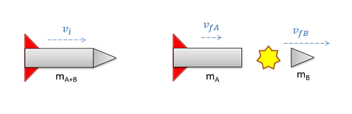
\[m_{A+B} v_i=m_A v_{f A}+m_B v_{f B}\]

When dealing with conservation of momentum problems, we will simply set up an equation setting the total initial momentum equal to the total final momentum. This will serve as the basis of analysis for many collisions, as is discussed in the following sections.

Video Lecture

Example \(\PageIndex{1}\)

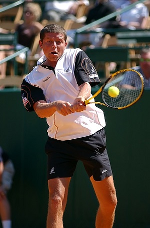
A tennis ball (0.06 kg) is served to a tennis player at a speed of 10 m/s. The player then returns the ball at a speed of 36 m/s.

• What is the impulse exerted on the ball?
• If a high-speed camera reveals the impact lasted 0.02 seconds, what is the average force exerted on the ball during the collision?

Figure \(\PageIndex{2}\): A player in a tennis match serves a ball.

Solution

Video \(\PageIndex{2}\): Worked solution to example problem \(\PageIndex{1}\), provided by Dr. Majid Chatsaz. YouTube source: https://youtu.be/WzD-ZyJy-T4.

Example \(\PageIndex{2}\)

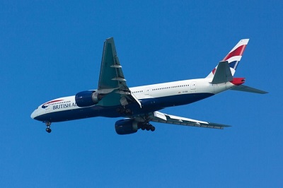
A plane with a mass of 80,000 kg is traveling at a velocity of 200 meters per second when the engines cut out. Twenty seconds later, it’s noticed that the velocity has dropped to 190 m/s. Assuming the plane is not gaining or losing altitude, what is the average drag force on the plane?

Figure \(\PageIndex{3}\): An airliner in flight.

Solution

Video \(\PageIndex{3}\): Worked solution to example problem \(\PageIndex{2}\), provided by Dr. Majid Chatsaz. YouTube source: https://youtu.be/dzhIT3r3u3k.

Example \(\PageIndex{3}\)

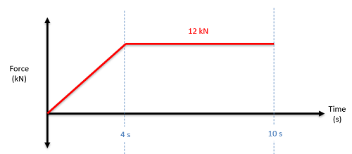
The plot below shows the thrust generated by the engine on a jet fighter (mass of 2500 kg) over ten seconds. If the plane is starting from rest on a runway, and friction and drag are negligible, determine the speed of the plane at the end of these ten seconds.

Figure \(\PageIndex{3}\): problem diagram for Example \(\PageIndex{3}\). Graph of the thrust force generated by a jet engine for the first 10 seconds of its motion starting from rest.

Solution

Video \(\PageIndex{4}\): Worked solution to example problem \(\PageIndex{3}\), provided by Dr. Majid Chatsaz. YouTube source: https://youtu.be/XGxVjLa6wqQ.