
4.5: Equivalent Point Load
- Page ID
- 52471

\( \newcommand{\vecs}[1]{\overset { \scriptstyle \rightharpoonup} {\mathbf{#1}} } \)
\( \newcommand{\vecd}[1]{\overset{-\!-\!\rightharpoonup}{\vphantom{a}\smash {#1}}} \)
\( \newcommand{\id}{\mathrm{id}}\) \( \newcommand{\Span}{\mathrm{span}}\)
( \newcommand{\kernel}{\mathrm{null}\,}\) \( \newcommand{\range}{\mathrm{range}\,}\)
\( \newcommand{\RealPart}{\mathrm{Re}}\) \( \newcommand{\ImaginaryPart}{\mathrm{Im}}\)
\( \newcommand{\Argument}{\mathrm{Arg}}\) \( \newcommand{\norm}[1]{\| #1 \|}\)
\( \newcommand{\inner}[2]{\langle #1, #2 \rangle}\)
\( \newcommand{\Span}{\mathrm{span}}\)
\( \newcommand{\id}{\mathrm{id}}\)
\( \newcommand{\Span}{\mathrm{span}}\)
\( \newcommand{\kernel}{\mathrm{null}\,}\)
\( \newcommand{\range}{\mathrm{range}\,}\)
\( \newcommand{\RealPart}{\mathrm{Re}}\)
\( \newcommand{\ImaginaryPart}{\mathrm{Im}}\)
\( \newcommand{\Argument}{\mathrm{Arg}}\)
\( \newcommand{\norm}[1]{\| #1 \|}\)
\( \newcommand{\inner}[2]{\langle #1, #2 \rangle}\)
\( \newcommand{\Span}{\mathrm{span}}\) \( \newcommand{\AA}{\unicode[.8,0]{x212B}}\)
\( \newcommand{\vectorA}[1]{\vec{#1}} % arrow\)
\( \newcommand{\vectorAt}[1]{\vec{\text{#1}}} % arrow\)
\( \newcommand{\vectorB}[1]{\overset { \scriptstyle \rightharpoonup} {\mathbf{#1}} } \)
\( \newcommand{\vectorC}[1]{\textbf{#1}} \)
\( \newcommand{\vectorD}[1]{\overrightarrow{#1}} \)
\( \newcommand{\vectorDt}[1]{\overrightarrow{\text{#1}}} \)
\( \newcommand{\vectE}[1]{\overset{-\!-\!\rightharpoonup}{\vphantom{a}\smash{\mathbf {#1}}}} \)
\( \newcommand{\vecs}[1]{\overset { \scriptstyle \rightharpoonup} {\mathbf{#1}} } \)
\( \newcommand{\vecd}[1]{\overset{-\!-\!\rightharpoonup}{\vphantom{a}\smash {#1}}} \)
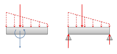
\(\newcommand{\avec}{\mathbf a}\) \(\newcommand{\bvec}{\mathbf b}\) \(\newcommand{\cvec}{\mathbf c}\) \(\newcommand{\dvec}{\mathbf d}\) \(\newcommand{\dtil}{\widetilde{\mathbf d}}\) \(\newcommand{\evec}{\mathbf e}\) \(\newcommand{\fvec}{\mathbf f}\) \(\newcommand{\nvec}{\mathbf n}\) \(\newcommand{\pvec}{\mathbf p}\) \(\newcommand{\qvec}{\mathbf q}\) \(\newcommand{\svec}{\mathbf s}\) \(\newcommand{\tvec}{\mathbf t}\) \(\newcommand{\uvec}{\mathbf u}\) \(\newcommand{\vvec}{\mathbf v}\) \(\newcommand{\wvec}{\mathbf w}\) \(\newcommand{\xvec}{\mathbf x}\) \(\newcommand{\yvec}{\mathbf y}\) \(\newcommand{\zvec}{\mathbf z}\) \(\newcommand{\rvec}{\mathbf r}\) \(\newcommand{\mvec}{\mathbf m}\) \(\newcommand{\zerovec}{\mathbf 0}\) \(\newcommand{\onevec}{\mathbf 1}\) \(\newcommand{\real}{\mathbb R}\) \(\newcommand{\twovec}[2]{\left[\begin{array}{r}#1 \\ #2 \end{array}\right]}\) \(\newcommand{\ctwovec}[2]{\left[\begin{array}{c}#1 \\ #2 \end{array}\right]}\) \(\newcommand{\threevec}[3]{\left[\begin{array}{r}#1 \\ #2 \\ #3 \end{array}\right]}\) \(\newcommand{\cthreevec}[3]{\left[\begin{array}{c}#1 \\ #2 \\ #3 \end{array}\right]}\) \(\newcommand{\fourvec}[4]{\left[\begin{array}{r}#1 \\ #2 \\ #3 \\ #4 \end{array}\right]}\) \(\newcommand{\cfourvec}[4]{\left[\begin{array}{c}#1 \\ #2 \\ #3 \\ #4 \end{array}\right]}\) \(\newcommand{\fivevec}[5]{\left[\begin{array}{r}#1 \\ #2 \\ #3 \\ #4 \\ #5 \\ \end{array}\right]}\) \(\newcommand{\cfivevec}[5]{\left[\begin{array}{c}#1 \\ #2 \\ #3 \\ #4 \\ #5 \\ \end{array}\right]}\) \(\newcommand{\mattwo}[4]{\left[\begin{array}{rr}#1 \amp #2 \\ #3 \amp #4 \\ \end{array}\right]}\) \(\newcommand{\laspan}[1]{\text{Span}\{#1\}}\) \(\newcommand{\bcal}{\cal B}\) \(\newcommand{\ccal}{\cal C}\) \(\newcommand{\scal}{\cal S}\) \(\newcommand{\wcal}{\cal W}\) \(\newcommand{\ecal}{\cal E}\) \(\newcommand{\coords}[2]{\left\{#1\right\}_{#2}}\) \(\newcommand{\gray}[1]{\color{gray}{#1}}\) \(\newcommand{\lgray}[1]{\color{lightgray}{#1}}\) \(\newcommand{\rank}{\operatorname{rank}}\) \(\newcommand{\row}{\text{Row}}\) \(\newcommand{\col}{\text{Col}}\) \(\renewcommand{\row}{\text{Row}}\) \(\newcommand{\nul}{\text{Nul}}\) \(\newcommand{\var}{\text{Var}}\) \(\newcommand{\corr}{\text{corr}}\) \(\newcommand{\len}[1]{\left|#1\right|}\) \(\newcommand{\bbar}{\overline{\bvec}}\) \(\newcommand{\bhat}{\widehat{\bvec}}\) \(\newcommand{\bperp}{\bvec^\perp}\) \(\newcommand{\xhat}{\widehat{\xvec}}\) \(\newcommand{\vhat}{\widehat{\vvec}}\) \(\newcommand{\uhat}{\widehat{\uvec}}\) \(\newcommand{\what}{\widehat{\wvec}}\) \(\newcommand{\Sighat}{\widehat{\Sigma}}\) \(\newcommand{\lt}{<}\) \(\newcommand{\gt}{>}\) \(\newcommand{\amp}{&}\) \(\definecolor{fillinmathshade}{gray}{0.9}\)An equivalent point load is a single point force that will have the same effect on a body as the original loading condition, which is usually a distributed force. The equivalent point load should always cause the same linear acceleration and angular acceleration as the original force it is equivalent to (or cause the same reaction forces if the body is constrained). Finding the equivalent point load for a distributed force often helps simplify the analysis of a system by removing the integrals from the equations of equilibrium or equations of motion in later analysis.
Finding the Equivalent Point Load
When finding the equivalent point load, we need to find the magnitude, direction, and point of application of a single force that is equivalent to the distributed force we are given. In this course we will only deal with distributed forces with a uniform direction, in which case the direction of the equivalent point load will match the uniform direction of the distributed force. This leaves the magnitude and the point of application to be found. There are two options available to find these values:
- We can find the magnitude and the point of application of the equivalent point load via integration of the force functions.
- We can use the area/volume and the centroid/center of volume of the area or volume under the force function.
The first method is more flexible, allowing us to find the equivalent point load for any force function that we can make a mathematical formula for (assuming we have the skill in calculus to integrate that function). The second method is usually faster, assuming that we can look up the values for the area or volume under the force curve and the values for the centroid or center of volume for the area under the curve.
Using Integration in 2D Surface Force Problems:
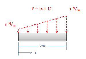
Finding the equivalent point load via integration always begins by determining the mathematical formula that is the force function. The force function mathematically relates the magnitude of the force \((F)\) to the position \((x)\). In this case the force is acting along a single line, so the position can be entirely determined by knowing the \(x\) coordinate, but in later problems we may also need to relate the magnitude of the force to the \(y\) and \(z\) coordinates. In our example above, we can relate magnitude of the force to the position by stating that the magnitude of the force at any point in Newtons per meter is equal to the \(x\) position in meters plus one.
The magnitude of the equivalent point load will be equal to the area under the force function. This will be the integral of the force function over its entire length (in this case, from \(x = 0\) to \(x = 2\)).
\[ F_{eq} = \int\limits_{x \, min}^{x \, max} F(x) \, dx \]
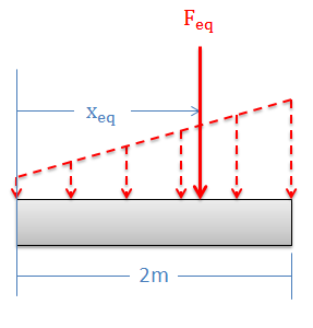
Now that we have the magnitude of the equivalent point load such that it matches the magnitude of the original force, we need to adjust the position \((x_{eq})\) such that it would cause the same moment as the original distributed force. The moment of the distributed force will be the integral of the force function \((F(x))\) times the moment arm about the origin \((x)\). The moment of the equivalent point load will be equal to the magnitude of the equivalent point load that we just found times the moment arm for the equivalent point load \((x_{eq})\). If we set these two things equal to one another and then solve for the position of the equivalent point load \((x_{eq})\) we are left with the following equation.
\[ x_{eq} = \frac{\int\limits_{x \, min}^{x \, max} (F(x) * x) \, dx}{F_{eq}} \]
Now that we have the magnitude, direction, and position of the equivalent point load, we can draw the point load in our original diagram. This point force can be used in place of the distributed force in further analysis.
Using the Area and Centroid in 2D Surface Force Problems:
As an alternative to using integration, we can use the area under the force curve and the centroid of the area under the force curve to find the equivalent point load's magnitude and point of application respectively.
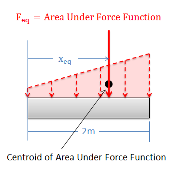
The magnitude \((F_{eq})\) of the equivalent point load will be equal to the area under the force function. We can find this area using calculus, but there are often easier geometry-based ways of finding the area under the force function.
The equivalent point load will also travel through centroid of the area under the force function. This allows us to find the value for \(x_{eq}\). The centroid for many common shapes can be looked up in tables, and the parallel axis theorem can be used to determine the centroid of more complex shapes (see the Appendix page on centroids for more details).
Using Integration in 3D Surface Force Problems:
With surface force in a 3D problem, the force is distributed over a surface, rather than along a single line. To find the magnitude of the equivalent point load we will again start by finding the mathematical equation for the force function. Because the force is distributed over an area rather than just a line, the magnitude of the force may be related to both the \(x\) and the \(y\) coordinate, rather than just the \(x\) coordinate as before.
The magnitude of the equivalent point load \((F_{eq})\) will be equal to the volume under the force curve. To calculate this value we will integrate the force function over the area that the force is applied to. To integrate this function \(F(x,y)\) in terms of the area, we will need to break the integral down further, integrating over \(x\) and then integrating over \(y\).
\[ F_{eq} = \int F(x,y) \, dA = \int\limits_{y \, min}^{y \, max} \left( \, \int\limits_{x \, min}^{x \, max} F(x,y) \, dx \right) \, dy \]
Once we solve for the magnitude of the equivalent point load, we can then solve for the position of the equivalent point load. Since the force is spread over a surface, we will need to calculate both the \(x\) \((x_{eq})\) and the \(y\) \((y_{eq})\) coordinates for the position. The process for solving for these values is similar to what was done with only an \(x\) value, except we change the moment arm value to match the equivalent point load coordinate we are looking for.
\[ x_{eq} = \frac{\int (F(x,y) * x) \, dA}{F_{eq}} \]
\[ y_{eq} = \frac{\int (F(x,y) * x) \, dA}{F_{eq}} \]
In each of the equations above, we will need to expand out the area integral into \(x\) and \(y\) integrals (as we did for \(F_{eq}\)) in order to be able to solve them.
Using Volume and Center of Volume in 3D Surface Force Problems:
Just as in the 2D problems, there are some available shortcuts to finding the equivalent point load in 3D surface force problems. For a force spread over an area, the magnitude \((F_{eq})\) of the equivalent point load will be equal to the volume under the force function. The equivalent point load will also travel through the center of volume of the volume under the force function. This should allow you to determine both \(x_{eq}\) and \(y_{eq}\).
The center of volume for a shape will be the same as the center of mass for a shape if the shape is assumed to have uniform density. It should be possible to look these values up for common shapes in a table. Again, the parallel axis theorem can be used to find the center of volume for more complex shapes (See the Center of Mass page in Appendix 2 for more details).
Using Integration in Body Force Problems:
When we jump to body forces, the magnitude of our force will vary with \(x\), \(y\), and \(z\) coordinates. This means that our force function can include all of these variables \((F(x,y,z))\). To find the magnitude of the equivalent point load we integrate over the volume, breaking the volume integral down into \(x\), \(y\), and then \(z\) integrals.
\begin{align} F_{eq} &= \int F(x,y,z) \, dV \\ &= \int\limits_{z \, min}^{z \, max} \left( \, \int\limits_{y \, min}^{y \, max} \left( \, \int\limits_{x \, min}^{x \, max} F(x,y,z) \, dx \right) \, dy \right) \, dz \end{align}
To find the point of application of the equivalent point load, we will need to find all three coordinate positions. To do this, we will expand out the equations we used with two coordinates to include the third coordinate \((z_{eq})\).
\[ x_{eq} = \frac{\int (F(x,y,z) * x) \, dV}{F_{eq}} \]
\[ y_{eq} = \frac{\int (F(x,y,z) * y) \, dV}{F_{eq}} \]
\[ z_{eq} = \frac{\int (F(x,y,z) * z) \, dV}{F_{eq}} \]
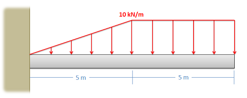
Example \(\PageIndex{1}\)
Determine the magnitude and the point of application for the equivalent point load of the distributed force shown below.
- Solution
-
Video \(\PageIndex{2}\): Worked solution to example problem \(\PageIndex{1}\), provided by Dr. Jacob Moore. YouTube source: https://youtu.be/h_E0XjIJaiI.
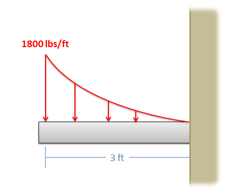
Example \(\PageIndex{2}\)
Determine the magnitude and the point of application for the equivalent point load of the distributed force shown below.
- Solution
-
Video \(\PageIndex{3}\): Worked solution to example problem \(\PageIndex{2}\), provided by Dr. Jacob Moore. YouTube source: https://youtu.be/D4JoQpOyI38.
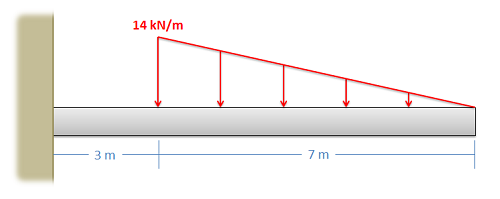
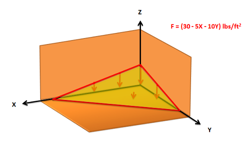
Example \(\PageIndex{3}\)
Determine the magnitude and the point of application for the equivalent point load of the distributed force shown below.
- Solution
-
Video \(\PageIndex{4}\): Worked solution to example problem \(\PageIndex{3}\), provided by Dr. Jacob Moore. YouTube source: https://youtu.be/UbnfNAQctyg.
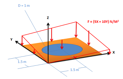
Example \(\PageIndex{4}\)
The wind has piled up sand into a corner on a building. The building supervisor is worried about the weight of the sand pushing against the roof of the basement below. The function describing force of the sand pushing down on the surface is given below. Find the magnitude, direction and point of application of the equivalent point load for the distributed force of the sand. Draw the equivalent point load in a diagram.
- Solution
-
Video \(\PageIndex{5}\): Worked solution to example problem \(\PageIndex{4}\), provided by Dr. Jacob Moore. YouTube source: https://youtu.be/IaSe_g3_Mgk.