10.4: Two-Dimensional Particle Collisions

Last updated
Save as PDF

Page ID: 54745

\( \newcommand{\vecs}[1]{\overset { \scriptstyle \rightharpoonup} {\mathbf{#1}} } \) \( \newcommand{\vecd}[1]{\overset{-\!-\!\rightharpoonup}{\vphantom{a}\smash {#1}}} \)\(\newcommand{\id}{\mathrm{id}}\) \( \newcommand{\Span}{\mathrm{span}}\) \( \newcommand{\kernel}{\mathrm{null}\,}\) \( \newcommand{\range}{\mathrm{range}\,}\) \( \newcommand{\RealPart}{\mathrm{Re}}\) \( \newcommand{\ImaginaryPart}{\mathrm{Im}}\) \( \newcommand{\Argument}{\mathrm{Arg}}\) \( \newcommand{\norm}[1]{\| #1 \|}\) \( \newcommand{\inner}[2]{\langle #1, #2 \rangle}\) \( \newcommand{\Span}{\mathrm{span}}\) \(\newcommand{\id}{\mathrm{id}}\) \( \newcommand{\Span}{\mathrm{span}}\) \( \newcommand{\kernel}{\mathrm{null}\,}\) \( \newcommand{\range}{\mathrm{range}\,}\) \( \newcommand{\RealPart}{\mathrm{Re}}\) \( \newcommand{\ImaginaryPart}{\mathrm{Im}}\) \( \newcommand{\Argument}{\mathrm{Arg}}\) \( \newcommand{\norm}[1]{\| #1 \|}\) \( \newcommand{\inner}[2]{\langle #1, #2 \rangle}\) \( \newcommand{\Span}{\mathrm{span}}\)\(\newcommand{\AA}{\unicode[.8,0]{x212B}}\)

To analyze collisions in two dimensions, we will need to adapt the methods we used for a single dimension. To start, the conservation of momentum equation will still apply to any type of collision.

\[ m_A \ \vec{v}_{A,f} + m_B \ \vec{v}_{B,f} = m_A \ \vec{v}_{A,i} + m_B \ \vec{v}_{B,i} \]

This is, of course, a vector equation, so we can break all those velocities into components to make our one vector equation into two scalar equations. In the equations below, we break the conservation of momentum equation into \(x\) and \(y\) components.

\[ m_A \ v_{A,f,x} + m_B \ v_{B,f,x} = m_A \ v_{A,i,x} + m_B \ v_{B,i,x} \]

\[ m_A \ v_{A,f,y} + m_B \ v_{B,f,y} = m_A \ v_{A,i,y} + m_B \ v_{B,i,y} \]

In the subscripts for the velocities, we label the particle (\(A\) or \(B\)), the pre or post collision state (\(i\) or \(f\)), and the component (\(x\) or \(y\)). This triple subscript can make things a bit crowded, but as long as you are methodical about labeling and reading these subscripts it is fairly straightforward. To help ease interpretation, it's recommended that you follow a consistent ordering in the subscripts, labeling body, then pre/post collision, then direction.

To supplement the conservation of momentum equations, we will again need to determine the type of collision, classifying the collision as inelastic (where the two particles stick together after impact) or elastic or semi-elastic (where the particles bounce off of one another).

Inelastic Collisions:

In the case of inelastic collisions, the bodies will have the same final velocity as a consequence of sticking together. Rolling this relationship into the above conservation of momentum equations, we wind up with the following equations. These modified equations are usually enough to solve for the unknowns in the equations.

\[ m_{(A+B)} \ v_{f,x} = m_A \ v_{A,i,x} + m_B \ v_{B,i,x} \]

\[ m_{(A+B)} \ v_{f,y} = m_A \ v_{A,i,y} + m_B \ v_{B,i,y} \]

Elastic and Semi-Elastic Collisions:

Unlike the inelastic collisions, elastic and semi-elastic collisions will have separate velocities for each of the bodies post-collision. With each body having separate \(x\) and \(y\) components, this represents four unknown variables. Assuming we know all starting conditions, we will need four separate equations to solve for all unknowns.

Unlike the conservation of momentum equation, the conservation of energy equation we would use for elastic collisions is not a vector equation and cannot be broken down into components. Instead we will need to look to the coefficient of restitution, and set it equal to 1 for elastic collisions.

To solve these problems, we will first need to set up a specific set of coordinate axes. These axes will be the tangential direction (along the plane of the collision) and the normal direction (perpendicular to the plane of the collision). An example of these directions is shown in the figure below.

Two billiard balls, the black 8-ball and the red 15-ball, are colliding. The 8-ball is located slightly more to the left and closer to the viewer, while the 15-ball is slightly more to the right and farther back in the plane of the screen. The 8-ball's velocity prior to the collision points up and to the right, while the 15-ball's velocity prior to the collision points down and to the right. The plane of contact between the two balls is therefore slanted, pointing down and to the right in the plane of the screen. The tangential axis points along this plane, and the normal axis points 90° counterclockwise of the tangential axis. — Figure \(\PageIndex{1}\): In a 2-D collision, it is important to identify the normal and tangential directions. The tangential direction will always be along the plane of impact while the normal direction will be perpendicular to the plane of contact.

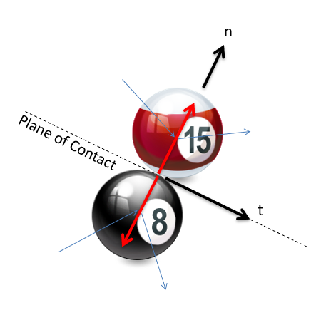
In examining the figure above, we can see something special about the tangential direction in that there are no forces on either body in this direction. With no forces, there is no impulse, and with no impulse there is no change in momentum for either particle individually in the tangential direction. This means that velocity is conserved for each body in the tangential direction on its own. Adding to that, momentum as a whole is conserved in the normal direction and the coefficient of restitution equation can be applied to the normal direction and we have the four equations we need to solve most problems.

\[ v_{A,f,t} = v_{A,i,t} \]

\[ v_{B,f,t} = v_{B,i,t} \]

\[ m_A \ v_{A,f,n} + m_B \ v_{B,f,n} = m_A \ v_{A,i,n} + m_B \ v_{B,i,n} \]

\[ \epsilon = - \frac{v_{A,f,n} - v_{B,f,n}}{v_{A,i,n} + v_{B,i,n}} \]

To use the above equations, we will need to break all known velocities down into \(n\) and \(t\) components, then simply plug those values in and solve the above equations. In the end we may also need to convert the found \(n\) and \(t\) velocity components into \(x\) and \(y\) components or magnitudes and directions.

Video lecture covering this section, delivered by Dr. Jacob Moore. YouTube source: https://youtu.be/iugmHb5fLMA.

Example \(\PageIndex{1}\)

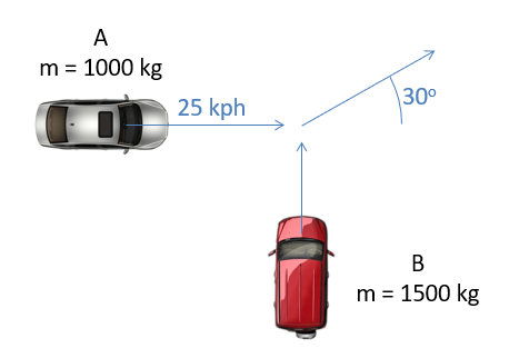
Two cars collide at an intersection as shown below. The cars become entangled with one another, sticking together after the impact. Based on the information given below on the initial velocities and assuming both cars slide away from the crash at the 30-degree angle as shown, what must the initial velocity of car B have been before the impact?

Car A, with a mass of 1000 kg, is on the upper left of the image, facing towards the right. It is moving towards the right at 25 kph. Car B, with a mass of 1500 kg, is in the lower middle of the image, facing towards the top of the image and moving in that direction. The two cars collide in the middle of the image and slide off upwards and to the right together, at a 30° angle above the horizontal. — Figure \(\PageIndex{2}\): problem diagram for Example \(\PageIndex{1}\). Two cars of different masses travel towards each other at right angles, colliding and becoming stuck together.

Solution: Video \(\PageIndex{2}\): Worked solution to example problem \(\PageIndex{1}\), provided by Dr. Majid Chatsaz. YouTube source: https://youtu.be/RBegCRhcGQc.

Example \(\PageIndex{2}\)

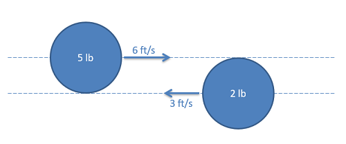
Two hockey pucks collide obliquely while sliding on a smooth surface, as shown below. Assume the coefficient of restitution is 0.7 and time of impact is 0.001s.

What is the final speed of each puck?
What is the average force exerted on each puck during the impact?

A uniformly circular 5-lb hockey puck in the upper left of the image is sliding directly towards the right at 6 ft/s. A uniformly circular 2-lb hockey puck in the lower right of the image, of the same radius as the 5-lb puck, is sliding directly towards the left at 3 ft/s. The direction of the 2-lb puck's motion places its center of mass in line with the lower edge of the 5-lb puck, and the upper edge of the 2-lb puck is in line with the center of mass of the 5-lb puck. — Figure \(\PageIndex{3}\): problem diagram for Example \(\PageIndex{2}\). Two hockey pucks of different masses but the same radius move towards each other, their centers of mass offset by a distance equal to the radius.

Solution: Video \(\PageIndex{3}\): Worked solution to example problem \(\PageIndex{2}\), provided by Dr. Majid Chatsaz. YouTube source: https://youtu.be/mRPjLk8RxQw.