6.5: Fatigue

Introduction

The concept of "fatigue" arose several times in the Module on Fracture (Module 23), as in the growth of cracks in the Comet aircraft that led to disaster when they became large enough to propagate catastrophically as predicted by the Griffith criterion. Fatigue, as understood by materials technologists, is a process in which damage accumulates due to the repetitive application of loads that may be well below the yield point. The process is dangerous because a single application of the load would not produce any ill effects, and a conventional stress analysis might lead to a assumption of safety that does not exist.

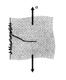
In one popular view of fatigue in metals, the fatigue process is thought to begin at an internal or surface flaw where the stresses are concentrated, and consists initially of shear flow along slip planes. Over a number of cycles, this slip generates intrusions and extrusions that begin to resemble a crack. A true crack running inward from an intrusion region may propagate initially along one of the original slip planes, but eventually turns to propagate transversely to the principal normal stress as seen in Figure 1.

Figure 1: Intrusion-extrusion model of fatigue crack initiation.

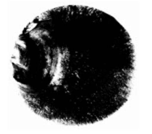
When the failure surface of a fatigued specimen is examined, a region of slow crack growth is usually evident in the form of a "clamshell" concentric around the location of the initial flf aw. (See Figure 2.) The clamshell region often contains concentric "beach marks" at which the crack was arrested for some number of cycles before resuming its growth. Eventually, the crack may become large enough to satisfy the energy or stress intensity criteria for rapid propagation, following the previous expressions for fracture mechanics. This final phase produces the rough surface typical of fast fracture. In postmortem examination of failed parts, it is often possible to correlate the beach marks with specific instances of overstress, and to estimate the applied stress at failure from the size of the crack just before rapid propagation and the fracture toughness of the material.

Figure 2: Typical fatigue-failure surfaces. From B. Chalmers, Physical Metallurgy, Wiley, p. 212, 1959.

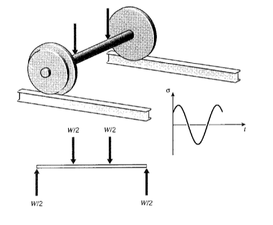
The modern study of fatigue is generally dated from the work of A. Wohler, a technologist in the German railroad system in the mid-nineteenth century. Wohler was concerned by the failure of axles after various times in service, at loads considerably less than expected. A railcar axle is essentially a round beam in four-point bending, which produces a compressive stress along the top surface and a tensile stress along the bottom (see Figure 3). After the axle has rotated a half turn, the bottom becomes the top and vice versa, so the stresses on a particular region of material at the surface varies sinusoidally from tension to compression and back again. This is now known as fully reversed fatigue loading.

Figure 3: Fatigue in a railcar axle.

S-N curves

Well before a microstructural understanding of fatigue processes was developed, engineers had developed empirical means of quantifying the fatigue process and designing against it. Perhaps the most important concept is the \(S-N\) diagram, such as those shown in Figure 4(H.W. Hayden, W.G. Moffatt, and J. Wulff, The Structure and Properties of Materials, Vol. III, John Wiley & Sons, 1965.), in which a constant cyclic stress amplitude \(S\) is applied to a specimen and the number of loading cycles \(N\) until the specimen fails is determined. Millions of cycles might be required to cause failure at lower loading levels, so the abscissa in usually plotted logarithmically.

Figure 4: \(S - N\) curves for aluminum and low-carbon steel.

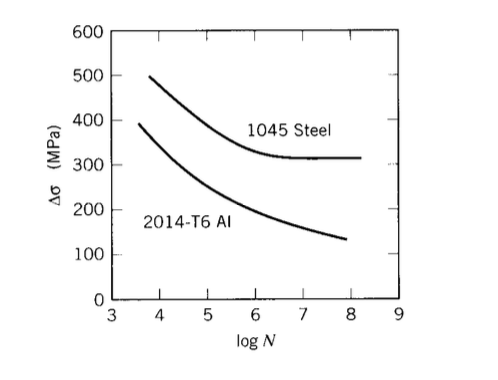
In some materials, notably ferrous alloys, the \(S - N\) curve flf attens out eventually, so that below a certain endurance limit \(\sigma_e\) failure does not occur no matter how long the loads are cycled. Obviously, the designer will size the structure to keep the stresses below \(\sigma_e\) by a suitable safety factor if cyclic loads are to be withstood. For some other materials such as aluminum, no endurance limit exists and the designer must arrange for the planned lifetime of the structure to be less than the failure point on the \(S - N\) curve.

Statistical variability is troublesome in fatigue testing; it is necessary to measure the lifetimes of perhaps twenty specimens at each of ten or so load levels to define the \(S - N\) curve with statistical confidence(A Guide for Fatigue Testing and the Statistical Analysis of Fatigue Data, ASTM STP-91-A, 1963.). It is generally impossible to cycle the specimen at more than approximately 10Hz (inertia in components of the testing machine and heating of the specimen often become problematic at higher speeds) and at that speed it takes 11.6 days to reach \(10^7\) cycles of loading. Obtaining a full \(S - N\) curve is obviously a tedious and expensive procedure.

Figure 5: Variability in fatigue lifetimes and fracture strengths.

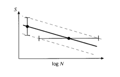
At first glance, the scatter in measured lifetimes seems enormous, especially given the log- arithmic scale of the abscissa. If the coefficient of variability in conventional tensile testing is usually only a few percent, why do the fatigue lifetimes vary over orders of magnitude? It must be remembered that in tensile testing, we are measuring the variability in stress at a given number of cycles (one), while in fatigue we are measuring the variability in cycles at a given stress. Stated differently, in tensile testing we are generating vertical scatter bars, but in fatigue they are horizontal (see Figure 5). Note that we must expect more variability in the lifetimes as the \(S - N\) curve becomes f atter, so that materials that are less prone to fatigue damage require more specimens to provide a given confidence limit on lifetime.

Effect of mean load

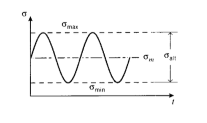
Of course, not all actual loading applications involve fully reversed stress cycling. A more general sort of fatigue testing adds a mean stress \(\sigma_m\) on which a sinusoidal cycle is superimposed, as shown in Figure 6. Such a cycle can be phrased in several ways, a common one being to state the alternating stress \(\sigma_{alt}\) and the stress ratio \(R = \sigma_{\min}/\sigma_{\max}\). For fully reversed loading, \(R = -1\). A stress cycle of \(R = 0.1\) is often used in aircraft component testing, and corresponds to a tension-tension cycle in which \(\sigma_{\min} = 0.1 \sigma_{\max}\).

Figure 6: Simultaneous mean and cyclic loading.

A very substantial amount of testing is required to obtain an \(S - N\) curve for the simple case of fully reversed loading, and it will usually be impractical to determine whole families of curves for every combination of mean and alternating stress. There are a number of strategems for finessing this difficulty, one common one being the Goodman diagram shown in Figure 7. Here a graph is constructed with mean stress as the abscissa and alternating stress as the ordinate, and a straight \lifeline" is drawn from \(\sigma_e\) on the \(\sigma_{alt}\) axis to the ultimate tensile stress \(\sigma_f\) on the \(\sigma_m\) axis. Then for any given mean stress, the endurance limit | the value of alternating stress at which fatigue fracture never occurs | can be read directly as the ordinate of the lifeline at that value of \(\sigma_m\). Alternatively, if the design application dictates a given ratio of \(\sigma_e\) to \(\sigma_{alt}\), a line is drawn from the origin with a slope equal to that ratio. Its intersection with the lifeline then gives the effective endurance limit for that combination of \(\sigma_f\) and \(\sigma_m\).

Figure 7: The Goodman diagram.

Miner's law for cumulative damage

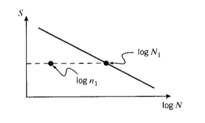
When the cyclic load level varies during the fatigue process, a cumulative damage model is often hypothesized. To illustrate, take the lifetime to be \(N_1\) cycles at a stress level \(\sigma_1\) and \(N_2\) at \(\sigma_2\). If damage is assumed to accumulate at a constant rate during fatigue and a number of cycles \(n_1\) is applied at stress \(\sigma_1\), where \(n_1 < N_1\) as shown in Figure 8, then the fraction of lifetime consumed will be \(n_1/N_1\). To determine how many additional cycles the specimen will survive at stress \(\sigma_2\), an additional fraction of life will be available such that the sum of the two fractions equals one:

\(\dfrac{n_1}{N_1} + \dfrac{n_2}{N_2} = 1\)

Note that absolute cycles and not log cycles are used here. Solving for the remaining cycles permissible at \(\sigma_2\):

 

The generalization of this approach is called Miner's Law, and can be written

\[\sum \dfrac{n_j}{N_j} = 1\]

where \(n_j\) is the number of cycles applied at a load corresponding to a lifetime of \(N_j\).

Example \(\PageIndex{1}\)

Consider a hypothetical material in which the \(S - N\) curve is linear from a value equal to the fracture stress \(\sigma_f\) at one cycle \((\log N = 0)\), falling to a value of \(\sigma_f/2\) at \(\log N = 7\) as shown in Figure 9. This behavior can be described by the relation

 

The material has been subjected to \(n_1 = 10^5\) load cycles at a level \(S = 0.6 \sigma_f\), and we wish to estimate how many cycles \(n_2\) the material can now withstand if we raise the load to \(S = 0.7 \sigma_f\). From the \(S - N\) relationship, we know the lifetime at \(S = 0.6 \sigma_f =\) constant would be \(N_1 = 3.98 \times 10^5\) and the lifetime at \(S = 0.7 \sigma_f =\) constant would be \(N-2 = 1.58 \times 10^4\). Now applying Equation 6.5.1:

Figure 9: Linear \(S - N\) curve.

\(\dfrac{n_1}{N_1} + \dfrac{n_2}{N_2} = \dfrac{1 \times 10^5}{3.98 \times 10^5} + \dfrac{n_2}{1.58 \times 10^4} = 1\)

\(n_2 = 1.18 \times 10^4\)

Miner's "law" should be viewed like many other material "laws," a useful approximation, quite easy to apply, that might be accurate enough to use in design. But damage accumulation in fatigue is usually a complicated mixture of several different mechanisms, and the assumption of linear damage accumulation inherent in Miner's law should be viewed skeptically. If portions of the material's microstructure become unable to bear load as fatigue progresses, the stress must be carried by the surviving microstructural elements. The rate of damage accumulation in these elements then increases, so that the material suffers damage much more rapidly in the last portions of its fatigue lifetime. If on the other hand cyclic loads induce strengthening mechanisms such as molecular orientation or crack blunting, the rate of damage accumulation could drop during some part of the material's lifetime. Miner's law ignores such effects, and often fails to capture the essential physics of the fatigue process.

Crack growth rates

Certainly in aircraft, but also in other structures as well, it is vital that engineers be able to predict the rate of crack growth during load cycling, so that the part in question be replaced or repaired before the crack reaches a critical length. A great deal of experimental evidence supports the view that the crack growth rate can be correlated with the cyclic variation in the stress intensity factor:

\[\dfrac{da}{dN} = A \Delta K^m\]

where \(da/dN\) is the fatigue crack growth rate per cycle, \(\Delta K = K_{\max} - K_{\min}\) is the stress intensity factor range during the cycle, and \(A\) and \(m\) are parameters that depend the material, environment, frequency, temperature and stress ratio. This is sometimes known as the "Paris law," and leads to plots similar to that shown in Figure 10.

Figure 10: The Paris law for fatigue crack growth rates.

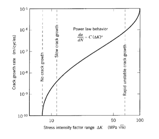
The exponent \(m\) is often near 4 for metallic systems, which might be rationalized as the damage accumulation being related to the volume \(V_p\) of the plastic zone: since the volume \(V_p\) of the zone scales with \(r_p^2\) and \(r_p \propto K_I^2\), then \(da/dn \propto \Delta K^4\). Some specific values of the constants \(m\) and \(A\) for various alloys in given in Table 1.

Table 1: Numerical parameters in the Paris equation.

alloy	\(m\)	\(A\)
Steel	3	\(10^{-11}\)
Aluminum	3	\(10^{-12}\)
Nickel	3.3	\(4 \times 10^{-12}\)
Titanium	5	\(10^{-11}\)

Exercise \(\PageIndex{1}\)

A steel has an ultimate tensile strength of 110 kpsi and a fatigue endurance limit of 50 kpsi. The load is such that the alternating stress is 0.4 of the mean stress. Using the Goodman method with a safety factor of 1.5, find the magnitude of alternating stress that gives safe operation.

Exercise \(\PageIndex{2}\)

A titanium alloy has an ultimate tensile strength of 120 kpsi and a fatigue endurance limit of 60 kpsi. The alternating stress is 20 kpsi. Find the allowable mean stress, using a safety factor of 2.

Exercise \(\PageIndex{3}\)

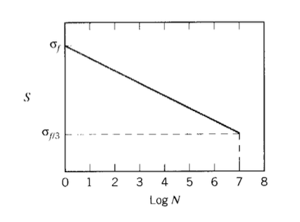
A material has an \(S - N\) curve that is linear from a value equal to the fracture stress \(\sigma_f\) at one cycle (\(\log N= 0\)), falling to a value of \(\sigma_f/3\) at \(\log N = 7\). The material has been subjected to \(n_1 = 1000\) load cycles at a level \(S = 0.7 \sigma_f\). Estimate how many cycles \(n_2\) the material can withstand if the stress amplitude is now raised to \(S = 0.8 \sigma_f\).

Exercise \(\PageIndex{4}\)

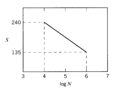
A steel alloy has an \(S - N\) curve that falls linearly from 240 kpsi at \(10^4\) cycles to 135 kpsi at \(10^6\) cycles. A specimen is loaded at 160 kpsi alternating stress for \(10^5\) cycles, after which the alternating stress is raised to 180 kpsi. How many additional cycles at this higher stress would the specimen be expected to survive?

Exercise \(\PageIndex{5}\)

Consider a body, large enough to be considered infinite in lateral dimension, containing a central through-thickness crack initially of length \(2a_0\) and subjected to a cyclic stress of amplitude \(\Delta \sigma\). Using the Paris Law (Equation 6.5.2), show that the number of cycles \(N_f\) needed for the crack to grow to a length \(2a_f\) is given by the relation

\(\ln (\dfrac{a_f}{a_0}) = A(\Delta \sigma)^2 \pi N_f\)

when \(m = 2\), and for other values of \(m\)

 

Exercise \(\PageIndex{6}\)

Use the expression obtained in Exercise \(\PageIndex{5}\) to compute the number of cycles a steel component can sustain before failure, where the initial crack halflength is 0.1 mm and the critical crack halflength to cause fracture is 2.5 mm. The stress amplitude per cycle is 950 MPa. Take the crack to be that of a central crack in an infinite plate.

Exercise \(\PageIndex{7}\)

Use the expression developed in Exercise \(PageIndex{1}\) to investigate whether it is better to limit the size \(a_0\) of initial flaws or to extend the size \(a_f\) of the flaw at which fast fracture occurs. Limiting \(a_0\) might be done with improved manufacturing or better inspection methods, and increasing \(a_f\) could be done by selecting a material with greater fracture toughness. For the "baseline" case, take \(m = 3.5, a_0 = 2\ mm\), \(a_f = mm\). Compute the percentage increase in \(N_f\) by letting (a) the initial f aw size to be reduced to \(a_0 = 1\ mm\), and (b) increasing the final f aw size to \(N_f = 10\ mm\).