1.1: One-dimensional Strain

Consider a prismatic, uniform thickness rod or beam of the initial length \(l_o\). The rod is fixed at one end and subjected a tensile force (Figure (\(\PageIndex{1}\))) at the other end. The current, deformed length is denoted by \(l\). The question is whether the resulting strain field is homogeneous or not. The concept of homogeneity in mechanics means independence of the solution on the spatial coordinates system, the rod axis in the present case. It can be shown that if the stress-strain curve of the material is convex or linear, the rod deforms uniformly and a homogeneous state of strains and stresses are developed inside the rod. This means that local and average strains are the same and the strain can be defined by considering the total lengths. The displacement at the fixed end \(x = 0\) of the rod is zero, \(u(x = 0)\) and the end displacement is

\[u(x = l) = l − l_o \label{1.1.1}\]

The strain is defined as a relative displacement. Relative to what? Initial, current length or something else? The definition of strain is simple but at the same time is non-unique.

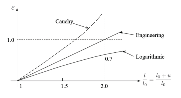
\[\epsilon \buildrel \rm {def} \over{=} \frac{l − l_o}{l_o} \text{ Engineering Strain} \label{1.1.2}\]

\[\epsilon \buildrel \rm {def} \over{=} \frac{1}{2} \frac{l^2 − l_o^2}{l^2} \text{ Cauchy Strain} \label{1.1.3}\]

\[\epsilon \buildrel \rm {def} \over{=} \ln \frac{l}{l_o} \text{ Logarithmic Strain} \label{1.1.4}\]

Each of the above three definitions satisfy the basic requirement that strain vanishes when \(l = l_o\) or \(u = 0\) and that strain in an increasing function of the displacement \(u\).

Consider a limiting case of Equation \ref{1.1.1} for small displacements \(\frac{u}{l_o} \ll 1\), for which \(l_o+l \approx 2l_o\) in Equation \ref{1.1.3}. Then, the Cauchy strain becomes

\[\epsilon = \frac{l − l_o}{l_o} \frac{l + l_o}{2l_o} \cong \frac{l − l_o}{l_o} \frac{2l}{2l_o} \cong \frac{l − l_o}{l_o} \label{1.1.5}\]

Thus, for small strain, the Cauchy strain reduces to the engineering strain. Likewise, expanding the expression for the logarithmic strain, Equation \ref{1.1.4} in Taylor series around \(l − l_o \cong 0\),

\[\left. \ln \frac{l}{l_o} \right|_{l/l_o=1} \cong \frac{l − l_o}{l_o} - \frac{1}{2} \left( \frac{l + l_o}{l_o} \right)^2 + \ldots \approx \frac{l − l_o}{l_o}\]

one can see that the logarithmic strain reduces to the engineering strain.

The plots of \(\epsilon\) versus \(\frac{l}{l_o}\) according to Equations \ref{1.1.2}-\ref{1.1.4} are shown in Figure (\(\PageIndex{1}\)).

Figure \(\PageIndex{1}\): Comparison of three definitions of the uniaxial strain.

Inhomogeneous Strain Field

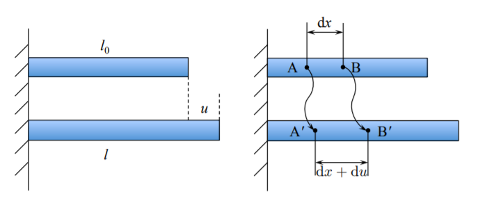
The strain must be defined locally and not for the entire structure. Consider an infinitesimal element \(dx\) in the undeformed configuration, Figure \(\PageIndex{2}\). After deformation the length of the original material element becomes \(dx + du\). The engineering strain is then

\[\epsilon_{\text{eng}} = \frac{(dx + du) − dx}{dx} = \frac{du}{dx} \label{1.1.7}\]

The spatial derivative of the displacement field is called the displacement gradient \(\boldsymbol{F} = \frac{du}{dx}\). For uniaxial state the strain is simply the displacement gradient. This is not true for general 3-D case.

Figure \(\PageIndex{2}\): Undeformed and deformed element in the homogenous and inhomogeneous strain field in the bar.

The local Cauchy strain is obtained by taking relative values of the difference of the square of the lengths. As shown in Equation \ref{1.1.5}, in order for the Cauchy strain to reduce to the engineering strain, the factor 2 must be introduced in the definition. Thus

\[\epsilon_c = \frac{1}{2} \frac{(dx + du)^2 − dx^2}{dx^2} = \frac{du}{dx} + \frac{1}{2} \left( \frac{du}{dx} \right)^2\]

or \(\epsilon_c = \boldsymbol{F} + \frac{1}{2} \boldsymbol{F}^2\). For small displacement gradients,

\[\epsilon_c = \epsilon_{\text{eng}}\]