Engineering LibreTexts

2.7: Complex Numbers

  • Page ID
    47958
    • Franz S. Hover & Michael S. Triantafyllou
    • Massachusetts Institute of Technology via MIT OpenCourseWare
    \( \newcommand{\vecs}[1]{\overset { \scriptstyle \rightharpoonup} {\mathbf{#1}} } \) \( \newcommand{\vecd}[1]{\overset{-\!-\!\rightharpoonup}{\vphantom{a}\smash {#1}}} \)\(\newcommand{\id}{\mathrm{id}}\) \( \newcommand{\Span}{\mathrm{span}}\) \( \newcommand{\kernel}{\mathrm{null}\,}\) \( \newcommand{\range}{\mathrm{range}\,}\) \( \newcommand{\RealPart}{\mathrm{Re}}\) \( \newcommand{\ImaginaryPart}{\mathrm{Im}}\) \( \newcommand{\Argument}{\mathrm{Arg}}\) \( \newcommand{\norm}[1]{\| #1 \|}\) \( \newcommand{\inner}[2]{\langle #1, #2 \rangle}\) \( \newcommand{\Span}{\mathrm{span}}\) \(\newcommand{\id}{\mathrm{id}}\) \( \newcommand{\Span}{\mathrm{span}}\) \( \newcommand{\kernel}{\mathrm{null}\,}\) \( \newcommand{\range}{\mathrm{range}\,}\) \( \newcommand{\RealPart}{\mathrm{Re}}\) \( \newcommand{\ImaginaryPart}{\mathrm{Im}}\) \( \newcommand{\Argument}{\mathrm{Arg}}\) \( \newcommand{\norm}[1]{\| #1 \|}\) \( \newcommand{\inner}[2]{\langle #1, #2 \rangle}\) \( \newcommand{\Span}{\mathrm{span}}\)\(\newcommand{\AA}{\unicode[.8,0]{x212B}}\)

    The complex number \(z = x + iy\) is interpreted as follows: the real part is \(x\), the imaginary part is \(y\), and \(i = \sqrt{−1}\) (imaginary). DeMoivre’s theorem connects complex \(z\) with the complex exponential. It states that \(cos \, \theta + i \, sin \, \theta = e^{i \theta}\), and so we can visualize any complex number in the two-dimensional plane, where the axes are the real part and the imaginary part. We say that \(Re(e^{i \theta}) = cos \, \theta\), and \(Im(e^{i \theta}) = sin \, \theta\), to denote the real and imaginary parts of a complex exponential. More generally, \(Re(z) = x\) and \(Im(z) = y\).
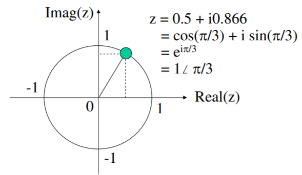
    Cartesian-plane graph representing a complex number in terms of the real part (x axis) and imaginary part (y axis)
    Figure \( \PageIndex{1}\): Imaginary number \(z\) represented as a graph on the Cartesian plane, with the x-axis representing the real part of \(z\) and the y-axis representing the imaginary part of \(z\).

    A complex number has a magnitude and an angle: \(|z| = \sqrt{x^2 + y^2}\), and arg \((z) = arctan2(y, x)\). We can refer to the \([x, y]\) description of \(z\) as Cartesian coordinates, whereas the [magnitude, angle] description is called polar coordinates. This latter is usually written as \(z = |z| \angle\) arg\((z)\). Arithmetic rules for two complex numbers \(z_1\) and \(z_2\) are as follows:

    \[\begin{align*} z_1 + z_2 &= (x_1 + x_2) + i (y_1 + y_2) \\[4pt] z_1 - z_2 &= (x_1 - x_2) + i (y_1 - y_2) \\[4pt] z_1 * z_2 &= |z_1| |z_2| \angle \arg (z_1) + \arg (z_2) \\[4pt] z_1 / z_2 &= \dfrac{|z_1|} {|z_2|} \angle \arg (z_1) - \arg (z_2) \end{align*}\]

    Note that, as given, addition and subtraction are most naturally expressed in Cartesian coordinates, and multiplication and division are cleaner in polar coordinates.


    This page titled 2.7: Complex Numbers is shared under a CC BY-NC-SA 4.0 license and was authored, remixed, and/or curated by Franz S. Hover & Michael S. Triantafyllou (MIT OpenCourseWare) via source content that was edited to the style and standards of the LibreTexts platform; a detailed edit history is available upon request.