5.1: Introduction to Short-Term Statistics

The spectrum contains information about the magnitude of each frequency component in a stationary and ergodic random process. A summation of harmonic functions with random phase satisfies ergodicity and stationarity, and this will be a dominant model of a random process in our discussion. Also, the central limit theorem provides that a random process of sufficient length and ensemble size has a Gaussian distribution.

The primary calculation is the frequency-domain multiplication of an input spectrum by a transfer function magnitude squared, so as to obtain the output spectrum. Further, a Gaussian input driving an LTI system will create a Gaussian output. Most importantly, the input and output spectra have statistical information that we will be able to integrate into the system design process. In this section, we focus on short-term statistics, namely those which will apply to a random process that is truly stationary. An easy example is a field of ocean waves: over the course of minutes or hours, the process is stationary, but over days the effects of distant storms will change the statistics.

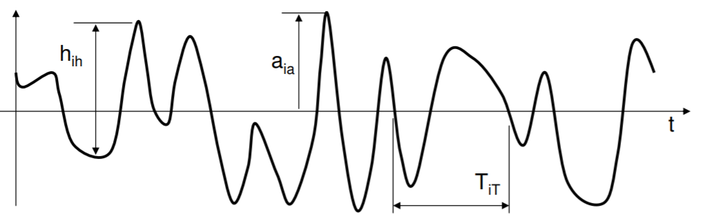
Considering specific ”events” within a random process, several of the most important are the amplitude \(a_{i_a}\), the height \(h_{i_h}\), and the period \(T_{i_T}\). The index here is counting through the record the number of amplitude measurements, height measurements, and period measurements. In the figure below, the period is measured specifically between zero downcrossings, and the amplitude is the maximum value reached after an upcrossing and before the next downcrossing. The height goes from the minimum after a zero downcrossing to the maximum after the following zero upcrossing. These definitions have to be applied consistently, because sometimes (as shown) there are fluctuations that do not cross over the zero line.

Figure \(\PageIndex{1}\): graph of a spectrum with the period \(T_{i_T}\) measured between zero downcrossings, the height \(h_{i_h}\) measured from the minimum after a zero downcrossing to the maximum after the next zero upcrosssing, and the amplitude \(a_{i_a}\) measured as the maximum value reached after an upcrossing and before the next downcrossing.

We will focus on statistics of the amplitude \(a\); the spectrum used below is that of \(a\). Let us define three even moments:

\begin{align} M_0 \, &= \int\limits_{0}^{\infty} S^+ (\omega) \, d\omega \\[4pt] M_2 \, &= \int\limits_{0}^{\infty} \omega^2 S^+ (\omega) \, d\omega \\[4pt] M_4 \, &= \int\limits_{0}^{\infty} \omega^4 S^+ (\omega) \, d\omega. \end{align}

We know already that \(M_0\) is related to the variance of the process. Without proof, these are combined into a ”bandwidth” parameter that we will use soon:

\[ \epsilon ^2 = 1 - \dfrac{M_2 ^2}{M_o M_4}. \]

Physically, \(\epsilon\) is near 1 if there are many local minima and maxima between zero crossings (broadband), whereas it is near zero if there is only one maxima after a zero upcrossing before returning to zero (narrow-band).