
6.4: Properties of the DTFS
- Page ID
- 103998

\( \newcommand{\vecs}[1]{\overset { \scriptstyle \rightharpoonup} {\mathbf{#1}} } \)
\( \newcommand{\vecd}[1]{\overset{-\!-\!\rightharpoonup}{\vphantom{a}\smash {#1}}} \)
\( \newcommand{\id}{\mathrm{id}}\) \( \newcommand{\Span}{\mathrm{span}}\)
( \newcommand{\kernel}{\mathrm{null}\,}\) \( \newcommand{\range}{\mathrm{range}\,}\)
\( \newcommand{\RealPart}{\mathrm{Re}}\) \( \newcommand{\ImaginaryPart}{\mathrm{Im}}\)
\( \newcommand{\Argument}{\mathrm{Arg}}\) \( \newcommand{\norm}[1]{\| #1 \|}\)
\( \newcommand{\inner}[2]{\langle #1, #2 \rangle}\)
\( \newcommand{\Span}{\mathrm{span}}\)
\( \newcommand{\id}{\mathrm{id}}\)
\( \newcommand{\Span}{\mathrm{span}}\)
\( \newcommand{\kernel}{\mathrm{null}\,}\)
\( \newcommand{\range}{\mathrm{range}\,}\)
\( \newcommand{\RealPart}{\mathrm{Re}}\)
\( \newcommand{\ImaginaryPart}{\mathrm{Im}}\)
\( \newcommand{\Argument}{\mathrm{Arg}}\)
\( \newcommand{\norm}[1]{\| #1 \|}\)
\( \newcommand{\inner}[2]{\langle #1, #2 \rangle}\)
\( \newcommand{\Span}{\mathrm{span}}\) \( \newcommand{\AA}{\unicode[.8,0]{x212B}}\)
\( \newcommand{\vectorA}[1]{\vec{#1}} % arrow\)
\( \newcommand{\vectorAt}[1]{\vec{\text{#1}}} % arrow\)
\( \newcommand{\vectorB}[1]{\overset { \scriptstyle \rightharpoonup} {\mathbf{#1}} } \)
\( \newcommand{\vectorC}[1]{\textbf{#1}} \)
\( \newcommand{\vectorD}[1]{\overrightarrow{#1}} \)
\( \newcommand{\vectorDt}[1]{\overrightarrow{\text{#1}}} \)
\( \newcommand{\vectE}[1]{\overset{-\!-\!\rightharpoonup}{\vphantom{a}\smash{\mathbf {#1}}}} \)
\( \newcommand{\vecs}[1]{\overset { \scriptstyle \rightharpoonup} {\mathbf{#1}} } \)
\( \newcommand{\vecd}[1]{\overset{-\!-\!\rightharpoonup}{\vphantom{a}\smash {#1}}} \)
\(\newcommand{\avec}{\mathbf a}\) \(\newcommand{\bvec}{\mathbf b}\) \(\newcommand{\cvec}{\mathbf c}\) \(\newcommand{\dvec}{\mathbf d}\) \(\newcommand{\dtil}{\widetilde{\mathbf d}}\) \(\newcommand{\evec}{\mathbf e}\) \(\newcommand{\fvec}{\mathbf f}\) \(\newcommand{\nvec}{\mathbf n}\) \(\newcommand{\pvec}{\mathbf p}\) \(\newcommand{\qvec}{\mathbf q}\) \(\newcommand{\svec}{\mathbf s}\) \(\newcommand{\tvec}{\mathbf t}\) \(\newcommand{\uvec}{\mathbf u}\) \(\newcommand{\vvec}{\mathbf v}\) \(\newcommand{\wvec}{\mathbf w}\) \(\newcommand{\xvec}{\mathbf x}\) \(\newcommand{\yvec}{\mathbf y}\) \(\newcommand{\zvec}{\mathbf z}\) \(\newcommand{\rvec}{\mathbf r}\) \(\newcommand{\mvec}{\mathbf m}\) \(\newcommand{\zerovec}{\mathbf 0}\) \(\newcommand{\onevec}{\mathbf 1}\) \(\newcommand{\real}{\mathbb R}\) \(\newcommand{\twovec}[2]{\left[\begin{array}{r}#1 \\ #2 \end{array}\right]}\) \(\newcommand{\ctwovec}[2]{\left[\begin{array}{c}#1 \\ #2 \end{array}\right]}\) \(\newcommand{\threevec}[3]{\left[\begin{array}{r}#1 \\ #2 \\ #3 \end{array}\right]}\) \(\newcommand{\cthreevec}[3]{\left[\begin{array}{c}#1 \\ #2 \\ #3 \end{array}\right]}\) \(\newcommand{\fourvec}[4]{\left[\begin{array}{r}#1 \\ #2 \\ #3 \\ #4 \end{array}\right]}\) \(\newcommand{\cfourvec}[4]{\left[\begin{array}{c}#1 \\ #2 \\ #3 \\ #4 \end{array}\right]}\) \(\newcommand{\fivevec}[5]{\left[\begin{array}{r}#1 \\ #2 \\ #3 \\ #4 \\ #5 \\ \end{array}\right]}\) \(\newcommand{\cfivevec}[5]{\left[\begin{array}{c}#1 \\ #2 \\ #3 \\ #4 \\ #5 \\ \end{array}\right]}\) \(\newcommand{\mattwo}[4]{\left[\begin{array}{rr}#1 \amp #2 \\ #3 \amp #4 \\ \end{array}\right]}\) \(\newcommand{\laspan}[1]{\text{Span}\{#1\}}\) \(\newcommand{\bcal}{\cal B}\) \(\newcommand{\ccal}{\cal C}\) \(\newcommand{\scal}{\cal S}\) \(\newcommand{\wcal}{\cal W}\) \(\newcommand{\ecal}{\cal E}\) \(\newcommand{\coords}[2]{\left\{#1\right\}_{#2}}\) \(\newcommand{\gray}[1]{\color{gray}{#1}}\) \(\newcommand{\lgray}[1]{\color{lightgray}{#1}}\) \(\newcommand{\rank}{\operatorname{rank}}\) \(\newcommand{\row}{\text{Row}}\) \(\newcommand{\col}{\text{Col}}\) \(\renewcommand{\row}{\text{Row}}\) \(\newcommand{\nul}{\text{Nul}}\) \(\newcommand{\var}{\text{Var}}\) \(\newcommand{\corr}{\text{corr}}\) \(\newcommand{\len}[1]{\left|#1\right|}\) \(\newcommand{\bbar}{\overline{\bvec}}\) \(\newcommand{\bhat}{\widehat{\bvec}}\) \(\newcommand{\bperp}{\bvec^\perp}\) \(\newcommand{\xhat}{\widehat{\xvec}}\) \(\newcommand{\vhat}{\widehat{\vvec}}\) \(\newcommand{\uhat}{\widehat{\uvec}}\) \(\newcommand{\what}{\widehat{\wvec}}\) \(\newcommand{\Sighat}{\widehat{\Sigma}}\) \(\newcommand{\lt}{<}\) \(\newcommand{\gt}{>}\) \(\newcommand{\amp}{&}\) \(\definecolor{fillinmathshade}{gray}{0.9}\)Introduction
In this module we will discuss the basic properties of the Discrete-Time Fourier Series. We will begin by refreshing your memory of our basic Fourier series equations:
\[f[n]=\sum_{k=0}^{N-1} c_{k} e^{j \omega_{0} k n} \nonumber \]
\[c_{k}=\frac{1}{\sqrt{N}} \sum_{n=0}^{N-1} f[n] e^{-\left(j \frac{2 \pi}{N} k n\right)} \nonumber \]
Let \(\mathscr{F}(\cdot)\) denote the transformation from \(f[n]\) to the Fourier coefficients
\[\mathscr{F}(f[n])=c_{k} \quad, \quad k \in \mathbb{Z} \nonumber \]
\(\mathscr{F}(\cdot)\) maps complex valued functions to sequences of complex numbers.
Linearity
\(\mathscr{F}(\cdot)\) is a linear transformation.
Theorem \(\PageIndex{1}\)
If \(\mathscr{F}(f[n])=c_{k}\) and \(\mathscr{F}(g[n])=d_{k}\). Then
\[\mathscr{F}(\alpha f[n])=\alpha c_{k} \quad, \quad \alpha \in \mathbb{C} \nonumber \]
and
\[\mathscr{F}(f[n]+g[n])=c_{k}+d_{k} \nonumber \]
Proof
Easy. Just linearity of integral.
\[\begin{align}
\mathscr{F}(f[n]+g[n]) &=\sum_{n=0}^{N}(f[n]+g[n]) e^{-\left(j \omega_{0} k n\right)}, k \in \mathbb{Z} \nonumber \\
&=\frac{1}{N} \sum_{n=0}^{N} f[n] e^{-\left(j \omega_{0} k n\right)}+\frac{1}{N} \sum_{n=0}^{N} g[n] e^{-\left(j \omega_{0} k n\right)}, k \in \mathbb{Z} \nonumber \\
&=c_{k}+d_{k}, k \in \mathbb{Z} \nonumber \\
&=c_{k}+d_{k}
\end{align} \nonumber \]
Shifting
Shifting in time equals a phase shift of Fourier coefficients.
Theorem \(\PageIndex{2}\)
\(\mathscr{F}\left(f\left[n-n_{0}\right]\right)=e^{-\left(j \omega_{0} k n_{0}\right)} c_{k}\) if \(c_{k}=\left|c_{k}\right| e^{j \angle\left(c_{k}\right)}\), then
\[\left|e^{-\left(j \omega_{0} k n_{0}\right)} c_{k}\right|=\left|e^{-\left(j \omega_{0} k n_{0}\right)}\right|\left|c_{k}\right|=\left|c_{k}\right| \nonumber \]
\[ \angle\left(e^{-\left(j \omega_{0} n_{0} k\right)}\right)=\angle\left(c_{k}\right)-\omega_{0} n_{0} k \nonumber \]
Proof
\[\begin{align}
\mathscr{F}\left(f\left[n-n_{0}\right]\right) &=\frac{1}{N} \sum_{n=0}^{N} f\left[n-n_{0}\right] e^{-\left(j \omega_{0} k n\right)}, \quad k \in \mathbb{Z} \nonumber \\
&=\frac{1}{N} \sum_{n=-n_{0}}^{N-n_{0}} f\left[n-n_{0}\right] e^{-\left(j \omega_{0} k\left(n-n_{0}\right)\right)} e^{-\left(j \omega_{0} k n_{0}\right)} \quad, \quad k \in \mathbb{Z} \nonumber \\
&=\frac{1}{N} \sum_{n=-n_{0}}^{N-n_{0}} f[\tilde{n}] e^{-\left(j \omega_{0} k \tilde{n}\right)} e^{-\left(j \omega_{0} k n_{0}\right)} \quad, \quad k \in \mathbb{Z} \nonumber \\
&=e^{-\left(j \omega_{0} k \tilde{n}\right)} c_{k} \quad, \quad k \in \mathbb{Z}
\end{align} \nonumber \]
Parseval's Relation
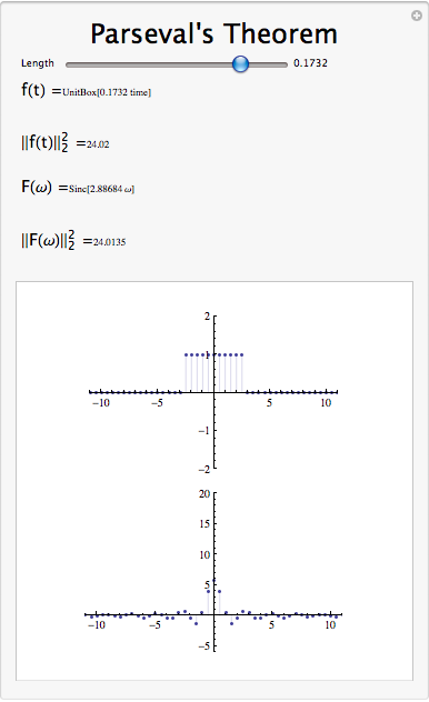
\[ \sum_{n=0}^{N}(|f[n]|)^{2}=N \sum_{k=0}^{N-1}\left(\left|c_{k}\right|\right)^{2} \nonumber \]
Parseval's relation tells us that the energy of a signal is equal to the energy of its Fourier transform.
Note
Parseval tells us that the Fourier series maps \(L^2[0,N]\) to \(l^2\).
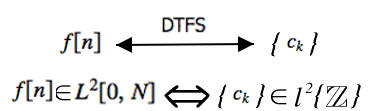
Figure \(\PageIndex{1}\)
Exercise \(\PageIndex{1}\)
For \(f[n]\) to have "finite energy," what do the \(c_k\) do as \( k \rightarrow \infty\)?
- Answer
-
\(\left(\left|c_{k}\right|\right)^{2}<\infty\) for \(f[n]\) to have finite energy.
Exercise \(\PageIndex{2}\)
If \(\forall k,|k|>0:\left(c_{k}=\frac{1}{k}\right)\), is \(f \in L^{2} [ [ 0, N ] ] \)?
- Answer
-
Yes, because \((|c_k|)^2=\frac{1}{k^2}\), which is summable.
Exercise \(\PageIndex{3}\)
Now, if \(\forall k,|k|>0:\left(c_{k}=\frac{1}{\sqrt{k}}\right)\), is \(f \in L^{2} [ [ 0, N ] ]\)?
- Answer
-
No, because \((|c_k|)^2=\frac{1}{k}\), which is not summable.
The rate of decay of the Fourier series determines if \(f[n]\) has finite energy.
ParsevalsTheorem Demonstration
Symmetry Properties
Rule \(\PageIndex{1}\): Even Signals
\(f[n] = f[-n]\)
\(\left\|c_{k}\right\|=\left\|c_{-k}\right\|\)
Proof
\(\begin{align}
c_{k}=&\frac{1}{N} \sum_{0}^{N}[n] \exp \left[-j \omega_{0} k n\right] \nonumber \\
=&\frac{1}{N} \sum_{0}^{\frac{N}{2}} f[n] \exp \left[-j \omega_{0} k n\right]+\frac{1}{N} \sum_{\frac{N}{2}}^{N} f[n] \exp \left[-j \omega_{0} k n\right] \nonumber \\
=&\frac{1}{N} \sum_{0}^{\frac{N}{2}} f[-n] \exp \left[-j \omega_{0} k n\right]+\frac{1}{N} \sum_{\frac{N}{2}}^{N} f[-n] \exp \left[-j \omega_{0} k n\right] \nonumber \\
=&\frac{1}{N} \sum_{0}^{N}[n]\left[\exp \left[j \omega_{0} k n\right]+\exp \left[-j \omega_{0} k n\right]\right] \nonumber \\
=&\frac{1}{N} \sum_{0}^{N}[n] 2 \cos \left[\omega_{0} k n\right]
\end{align}\)
Rule \(\PageIndex{2}\): Odd Signals
\(f[n]=-f[-n]\)
\(c_{k}=c_{-k}^*\)
Proof
\(\begin{align}
c_{k}=&\frac{1}{N} \sum_{0}^{N} f[n] \exp \left[-\mathrm{j} \omega_{0} k n\right] \nonumber \\
=&\frac{1}{N} \sum_{0}^{\frac{N}{2}} f[n] \exp \left[-\mathrm{j} \omega_{0} k n\right]+\frac{1}{N} \sum_{\frac{N}{2}}^{N} f[n] \exp \left[-\mathrm{j} \omega_{0} k n\right] \nonumber \\
=&\frac{1}{N} \sum_{0}^{\frac{N}{2}} f[n] \exp \left[-\mathrm{j} \omega_{0} k n\right]-\frac{1}{N} \sum_{\frac{N}{2}}^{N} f[-n] \exp \left[\mathrm{j} \omega_{0} k n\right] \nonumber \\
=&-\frac{1}{N} \sum_{0}^{N} f[n]\left[\exp \left[\mathrm{j} \omega_{0} k n\right]-\exp \left[-\mathrm{j} \omega_{0} k n\right]\right] \nonumber \\
=&-\frac{1}{N} \sum_{0}^{N} f[n] 2 \operatorname{j \sin}\left[\omega_{0} k n\right]
\end{align}\)
Rule \(\PageIndex{3}\): Real Signals
\(f[n] = f^*[n]\)
\(c_k = c_{-k}^*\)
Proof
\(\displaystyle{\begin{align}
c_{k}=&\frac{1}{N} \sum_{0}^{N} f[n] \exp \left[-\mathrm{j} \omega_{0} k n\right] \nonumber \\
=&\frac{1}{N} \sum_{0}^{\frac{N}{2}} f[n] \exp \left[-\mathrm{j} \omega_{0} k n\right]+\frac{1}{N} \sum_{\frac{N}{2}}^{N} f[n] \exp \left[-\mathrm{j} \omega_{0} k n\right] \nonumber \\
=&\frac{1}{N} \sum_{0}^{\frac{N}{2}} f[-n] \exp \left[-\mathrm{j} \omega_{0} k n\right]+\frac{1}{N} \sum_{\frac{N}{2}}^{N} f[-n] \exp \left[-\mathrm{j} \omega_{0} k n\right] \nonumber \\
=&\frac{1}{N} \sum_{0}^{N} f[n]\left[\exp \left[\mathrm{j} \omega_{0} k n\right]+\exp \left[-\mathrm{j} \omega_{0} k n\right]\right] \nonumber \\
=&\frac{1}{N} \sum_{0}^{N} f[n] 2 \cos \left[\omega_{0} k n\right]
\end{align}}\)
Differentiation in Fourier Domain
\[\left(\mathscr{F}(f[n])=c_{k}\right) \Rightarrow\left(\mathscr{F}\left(\frac{\mathrm{d} f[n]}{\mathrm{d} n}\right)=j k \omega_{0} c_{k}\right) \nonumber \]
Since
\[f[n]=\sum_{i=0}^{N} c_{k} e^{j \omega_{0} k n} \nonumber \]
then
\[\begin{align}
\frac{\mathrm{d}}{\mathrm{dn}} f[n] &=\sum_{k=0}^{N} c_{k} \frac{\mathrm{d} e^{j \omega_0 k n}}{\mathrm{dn}} \nonumber \\
&=\sum_{k=0}^{N} c_{k} j \omega_{0} k e^{j \omega_{0} k n}
\end{align} \nonumber \]
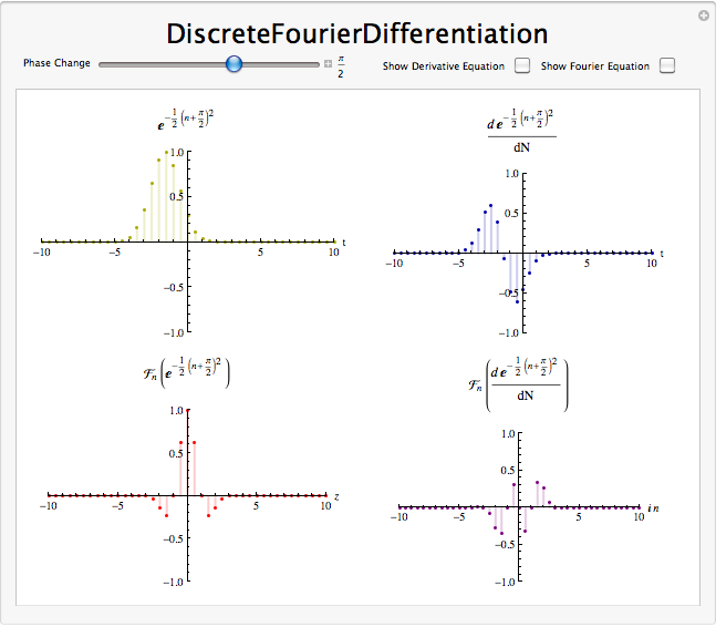
A differentiator attenuates the low frequencies in \(f[n]\) and accentuates the high frequencies. It removes general trends and accentuates areas of sharp variation.
Note
A common way to mathematically measure the smoothness of a function \(f[n]\) is to see how many derivatives are finite energy.
This is done by looking at the Fourier coefficients of the signal, specifically how fast they decay as \(k \rightarrow \infty\). If \(\mathscr{F}(f[n])=c_{k}\) and \(|c_k|\) has the form \(\frac{1}{k^l}\), then \(\mathscr{F}\left(\frac{\mathrm{d}^{m} f[n]}{\mathrm{d} n^{m}}\right)=\left(j k \omega_{0}\right)^{m} c_{k}\) and has the form \(\frac{k^m}{k^l}\). So for the \(m\)th derivative to have finite energy, we need
\[\sum_{k}\left(\left|\frac{k^{m}}{k^{l}}\right|\right)^{2}<\infty \nonumber \]
thus \(\frac{k^{m}}{k^{l}}\) decays faster than \(\frac{1}{k}\) which implies that
\[2l - 2m > 1 \nonumber \]
or
\[l > \frac{2m+1}{2} \nonumber \]
Thus the decay rate of the Fourier series dictates smoothness.
Fourier Differentiation Demo
Integration in the Fourier Domain
If
\[\mathscr{F}(f[n])=c_{k} \nonumber \]
then
\[\mathscr{F}\left(\sum_{\eta=0}^{n} f[\eta]\right)=\frac{1}{j \omega_{0} k} c_{k} \nonumber \]
Note
If \(c_0 \neq 0\), this expression doesn't make sense.
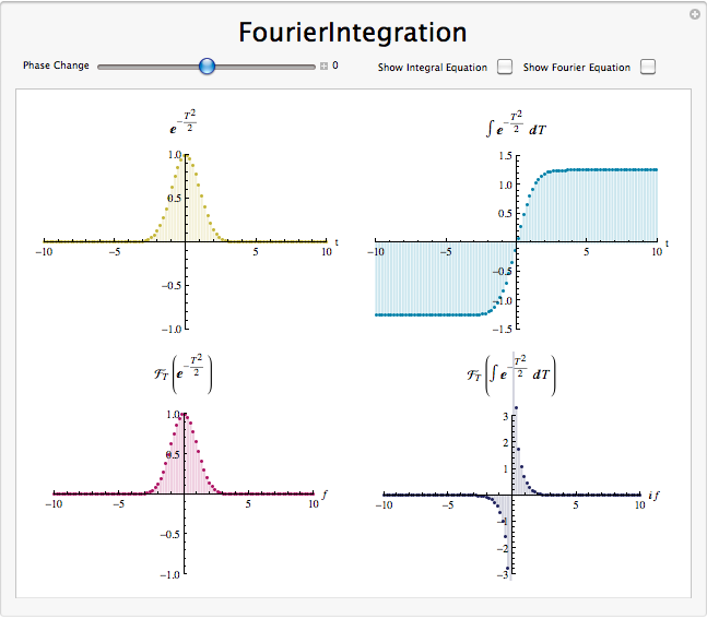
Integration accentuates low frequencies and attenuates high frequencies. Integrators bring out the general trends in signals and suppress short term variation (which is noise in many cases). Integrators are much nicer than differentiators.
Fourier Integration Demo
Signal Multiplication
Given a signal \(f[n]\) with Fourier coefficients \(c_k\) and a signal \(g[n]\) with Fourier coefficients \(d_k\), we can define a new signal, \(y[n]\), where \(y[n]=f[n]g[n]\). We find that the Fourier Series representation of \(y[n]\), \(e_k\), is such that \(e_{k}=\sum_{l=0}^{N} c_{l} d_{k-l}\). This is to say that signal multiplication in the time domain is equivalent to discrete-time circular convolution (Section 4.3) in the frequency domain. The proof of this is as follows
\[\begin{align}
e_{k} &=\frac{1}{N} \sum_{n=0}^{N} f[n] g[n] e^{-\left(j \omega_{0} k n\right)} \nonumber \\
&=\frac{1}{N} \sum_{n=0}^{N} \sum_{l=0}^{N} c_{l} e^{j \omega_{0} l n} g[n] e^{-\left(j \omega_{0} k n\right)} \nonumber \\
&=\sum_{l=0}^{N} c_{l}\left(\frac{1}{N} \sum_{n=0}^{N} g[n] e^{-\left(j \omega_{0}(k-l) n\right)}\right) \nonumber \\
&=\sum_{l=0}^{N} c_{l} d_{k-l}
\end{align} \nonumber \]
Conclusion
Like other Fourier transforms, the DTFS has many useful properties, including linearity, equal energy in the time and frequency domains, and analogs for shifting, differentation, and integration.
| Property | Signal | DTFS |
|---|---|---|
| Linearity | \(ax(n)+by(n)\) | \(aX(k)+bY(k)\) |
| Time Shifting | \(x(n−m)\) | \(X(k)e^{−j2 \pi mk/N}\) |
| Time Modulation | \(x(n) e^{j 2 \pi m n / N}\) | \(X(k−m)\) |
| Multiplication | \(x(n)y(n)\) | \(X(k)*Y(k)\) |
| Circular Convolution | \(x(n)*y(n)\) | \(X(k)Y(K)\) |