
6.5: Discrete Time Circular Convolution and the DTFS


- Last updated
- Jun 4, 2024
- Save as PDF

( \newcommand{\kernel}{\mathrm{null}\,}\)
Introduction
This module relates circular convolution of periodic signals in one domain to multiplication in the other domain.
You should be familiar with Discrete-Time Convolution (Section 4.3), which tells us that given two discrete-time signals x[n], the system's input, and h[n], the system's response, we define the output of the system as
\begin{align} y[n] &=x[n] * h[n] \nonumber \\ &=\sum_{k=-\infty}^{\infty} x[k] h[n-k] \end{align} \nonumber
When we are given two DFTs (finite-length sequences usually of length N), we cannot just multiply them together as we do in the above convolution formula, often referred to as linear convolution. Because the DFTs are periodic, they have nonzero values for n≥N and thus the multiplication of these two DFTs will be nonzero for n≥N. We need to define a new type of convolution operation that will result in our convolved signal being zero outside of the range n={0,1,…,N−1}. This idea led to the development of circular convolution, also called cyclic or periodic convolution.
Signal Circular Convolution
Given a signal f[n] with Fourier coefficients c_k and a signal g[n] with Fourier coefficients d_k, we can define a new signal, v[n], where v[n]=f[n] \circledast g[n]. We find that the Fourier Series representation of v[n], a_k, is such that a_k=c_kd_k. f[n] \circledast g[n] is the circular convolution (Section 7.5) of two periodic signals and is equivalent to the convolution over one interval, i.e. \displaystyle{f[n] \circledast g[n] = \sum_{n=0}^{N} \sum_{\eta=0}^{N} f[\eta] g[n-\eta]}.
Note
Circular convolution in the time domain is equivalent to multiplication of the Fourier coefficients.
This is proved as follows
\begin{align} a_{k} &=\frac{1}{N} \sum_{n=0}^{N} v[n] e^{-\left(j \omega_{0} k n\right)} \nonumber \\ &=\frac{1}{N^{2}} \sum_{n=0}^{N} \sum_{n=0}^{\eta} f[\eta] g[n-\eta] e^{-\left(j \omega_{0} k n\right)} \nonumber \\ &=\frac{1}{N} \sum_{\eta=0}^{N} f[\eta]\left(\frac{1}{N} \sum_{n=0}^{N} g[n-\eta] e^{-\left(j \omega_{0} k n\right)}\right) \nonumber \\ &=\left(\frac{1}{N} \sum_{\eta=0}^{N} f[\eta]\left(\frac{1}{N} \sum_{\nu=-\eta}^{N-\eta} g[\nu] e^{-\left(j \omega_{0}(\nu+\eta)\right)}\right)\right) \quad , \quad \nu = n - \eta \nonumber \\ &=\frac{1}{N} \sum_{\eta=0}^{N} f[\eta]\left(\frac{1}{N} \sum_{\nu=-\eta}^{N-\eta} g[\nu] e^{-\left(j \omega_{0} k \nu\right)}\right) e^{-\left(j \omega_{0} k \eta\right)} \nonumber \\ &=\frac{1}{N} \sum_{\eta=0}^{N} f[\eta] d_{k} e^{-\left(j \omega_{0} k \eta\right)} \nonumber \\ &=d_{k}\left(\frac{1}{N} \sum_{\eta=0}^{N} f[\eta] e^{-\left(j \omega_{0} k \eta\right)}\right) \nonumber \\ &=c_{k} d_{k} \end{align} \nonumber
Circular Convolution Formula
What happens when we multiply two DFT's together, where Y[k] is the DFT of y[n]?
Y[k] = F[k]H[k] \nonumber
when 0≤k≤N−1
Using the DFT synthesis formula for y[n]
y[n]=\frac{1}{N} \sum_{k=0}^{N-1} F[k] H[k] e^{j \frac{2 \pi}{N} k n} \nonumber
And then applying the analysis formula F[k]=\sum_{m=0}^{N-1} f[m] e^{(-j) \frac{2 \pi}{N} k n}
\begin{align} y[n] &=\frac{1}{N} \sum_{k=0}^{N-1} \sum_{m=0}^{N-1} f[m] e^{(-j) \frac{2 \pi}{N} k n} H[k] e^{j \frac{2 \pi}{N} k n} \nonumber \\ &=\sum_{m=0}^{N-1} f[m]\left(\frac{1}{N} \sum_{k=0}^{N-1} H[k] e^{j \frac{2 \pi}{N} k(n-m)}\right) \end{align} \nonumber
where we can reduce the second summation found in the above equation into h\left[((n-m))_{N}\right]=\frac{1}{N} \sum_{k=0}^{N-1} H[k] e^{j \frac{2 \pi}{N} k(n-m)} y[n]=\sum_{m=0}^{N-1} f[m] h\left[((n-m))_{N}\right] which equals circular convolution! When we have 0≤n≤N−1 in the above, then we get:
y[n] \equiv f[n] \circledast h[n] \nonumber
Note
The notation \circledast represents cyclic convolution "mod N".
Alternative Convolution Formula
Alternative Circular Convolution Algorithm
- Step 1: Calculate the DFT of f[n] which yields F[k] and calculate the DFT of h[n] which yields H[k].
- Step 2: Pointwise multiply Y[k]=F[k]H[k]
- Step 3: Inverse DFT Y[k] which yields y[n]
Seems like a roundabout way of doing things, but it turns out that there are extremely fast ways to calculate the DFT of a sequence.
To circularly convolve 2 N-point sequences: y[n]=\sum_{m=0}^{N-1} f[m] h\left[((n-m))_{N}\right]. For each n : N multiples, N−1 additions.
N points implies N^2 multiplications, N(N−1) additions implies O(N^2) complexity.
Steps for Circular Convolution
We can picture periodic (Section 6.1) sequences as having discrete points on a circle as the domain
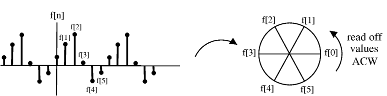
Figure \PageIndex{1}
Shifting by m, f(n+m), corresponds to rotating the cylinder m notches ACW (counter clockwise). For m=−2, we get a shift equal to that in the following illustration:
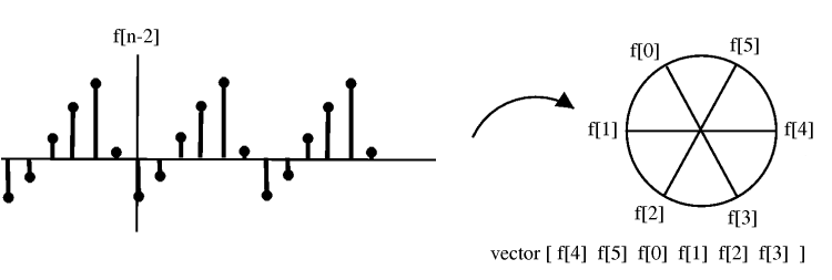
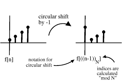
Figure \PageIndex{3}
To cyclic shift we follow these steps:
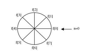
1) Write f(n) on a cylinder, ACW

2) To cyclic shift by m, spin cylinder m spots ACW
f[n] \rightarrow f\left[((n+m))_{N}\right] \nonumber
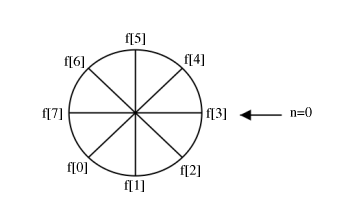
Notes on circular shifting
f[((n+N))_N]=f[n] Spinning N spots is the same as spinning all the way around, or not spinning at all.
f[((n+N))_N]=f[((n−(N−m)))_N] Shifting ACW mm is equivalent to shifting CW N−m
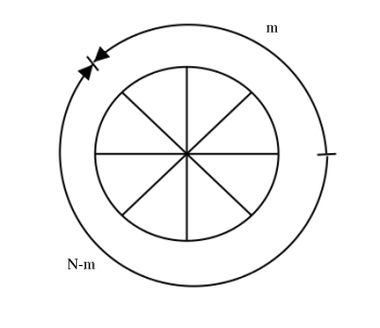
Figure \PageIndex{6}
f[((−n))_N] The above expression, simply writes the values of f[n] clockwise.
(a) f[n]
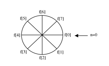
(b) f[((−n))_N]
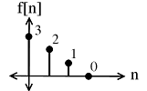
Example \PageIndex{1}
Convolve (n = 4)
 (a)
(a)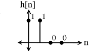 (b)
(b)- h[((−(m()()_N]
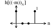
Figure \PageIndex{9}
Multiply f[m] and sum to yield: y[0]=3
- h[((1(−(m()()_N]
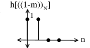
Figure \PageIndex{10}
Multiply f[m] and sum to yield: y[1]=5
- h[((2(−(m()()_N]
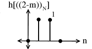
Figure \PageIndex{11}
Multiply f[m] and sum to yield: y[2]=3
- h[((3(−(m()()_N]
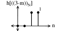
Figure \PageIndex{12}
Multiply f[m] and sum to yield: y[3]=1
Exercise
Take a look at a square pulse with a period of T.
For this signal c_{k}=\left\{\begin{array}{l} \frac{1}{N} \text { if } k=0 \\ \frac{1}{2} \frac{\sin \left(\frac{\pi}{2} k\right)}{\frac{\pi}{2} k} \text { otherwise } \end{array}\right.
Take a look at a triangle pulse train with a period of T.
This signal is created by circularly convolving the square pulse with itself. The Fourier coefficients for this signal are a_{k}=c_{k}^{2}=\frac{1}{4} \frac{\sin ^{2}}{\left(\frac{x}{2} k\right)}
Exercise \PageIndex{1}
Find the Fourier coefficients of the signal that is created when the square pulse and the triangle pulse are convolved.
- Answer
-
a_{k}=\left\{\begin{array}{ll} \text { undefined } & k=0 \\ \frac{1}{8} \frac{\sin ^{3}\left[\frac{\pi}{2} k\right]}{\left[\frac{\pi}{2} k\right]^{3}} & \text { otherwise } \end{array}\right.
Circular Shifts and the DFT
Theorem \PageIndex{1}: Circular Shifts and DFT
If f[n] \stackrel{\mathrm{DFT}}{\longleftrightarrow} F[k] then f\left[((n-m))_{N}\right] \stackrel{\mathrm{DFT}}{\longleftrightarrow} e^{-\left(j \frac{2 \pi}{N} k m\right)} F[k] (i.e. circular shift in time domain = phase shift in DFT)
Proof
f[n]=\frac{1}{N} \sum_{k=0}^{N-1} F[k] e^{j \frac{2 \pi}{N} k n} \nonumber
so phase shifting the DFT
\begin{align} f[n] &=\frac{1}{N} \sum_{k=0}^{N-1} F[k] e^{-\left(j \frac{2 \pi}{N} k n\right)} e^{j \frac{2 \pi}{N} k n} \nonumber \\ &=\frac{1}{N} \sum_{k=0}^{N-1} F[k] e^{j \frac{2 \pi}{N} k(n-m)} \nonumber \\ &=f\left[((n-m))_{N}\right] \end{align}
Circular Convolution Demonstration
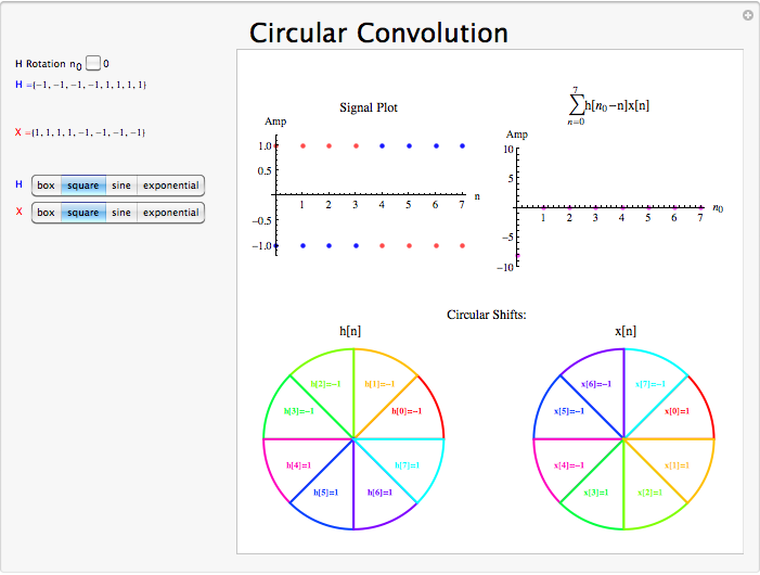
Conclusion
Circular convolution in the time domain is equivalent to multiplication of the Fourier coefficients in the frequency domain.