Chapter 2: Statics
- Page ID
- 103962
\( \newcommand{\vecs}[1]{\overset { \scriptstyle \rightharpoonup} {\mathbf{#1}} } \)
\( \newcommand{\vecd}[1]{\overset{-\!-\!\rightharpoonup}{\vphantom{a}\smash {#1}}} \)
\( \newcommand{\dsum}{\displaystyle\sum\limits} \)
\( \newcommand{\dint}{\displaystyle\int\limits} \)
\( \newcommand{\dlim}{\displaystyle\lim\limits} \)
\( \newcommand{\id}{\mathrm{id}}\) \( \newcommand{\Span}{\mathrm{span}}\)
( \newcommand{\kernel}{\mathrm{null}\,}\) \( \newcommand{\range}{\mathrm{range}\,}\)
\( \newcommand{\RealPart}{\mathrm{Re}}\) \( \newcommand{\ImaginaryPart}{\mathrm{Im}}\)
\( \newcommand{\Argument}{\mathrm{Arg}}\) \( \newcommand{\norm}[1]{\| #1 \|}\)
\( \newcommand{\inner}[2]{\langle #1, #2 \rangle}\)
\( \newcommand{\Span}{\mathrm{span}}\)
\( \newcommand{\id}{\mathrm{id}}\)
\( \newcommand{\Span}{\mathrm{span}}\)
\( \newcommand{\kernel}{\mathrm{null}\,}\)
\( \newcommand{\range}{\mathrm{range}\,}\)
\( \newcommand{\RealPart}{\mathrm{Re}}\)
\( \newcommand{\ImaginaryPart}{\mathrm{Im}}\)
\( \newcommand{\Argument}{\mathrm{Arg}}\)
\( \newcommand{\norm}[1]{\| #1 \|}\)
\( \newcommand{\inner}[2]{\langle #1, #2 \rangle}\)
\( \newcommand{\Span}{\mathrm{span}}\) \( \newcommand{\AA}{\unicode[.8,0]{x212B}}\)
\( \newcommand{\vectorA}[1]{\vec{#1}} % arrow\)
\( \newcommand{\vectorAt}[1]{\vec{\text{#1}}} % arrow\)
\( \newcommand{\vectorB}[1]{\overset { \scriptstyle \rightharpoonup} {\mathbf{#1}} } \)
\( \newcommand{\vectorC}[1]{\textbf{#1}} \)
\( \newcommand{\vectorD}[1]{\overrightarrow{#1}} \)
\( \newcommand{\vectorDt}[1]{\overrightarrow{\text{#1}}} \)
\( \newcommand{\vectE}[1]{\overset{-\!-\!\rightharpoonup}{\vphantom{a}\smash{\mathbf {#1}}}} \)
\( \newcommand{\vecs}[1]{\overset { \scriptstyle \rightharpoonup} {\mathbf{#1}} } \)
\(\newcommand{\longvect}{\overrightarrow}\)
\( \newcommand{\vecd}[1]{\overset{-\!-\!\rightharpoonup}{\vphantom{a}\smash {#1}}} \)
\(\newcommand{\avec}{\mathbf a}\) \(\newcommand{\bvec}{\mathbf b}\) \(\newcommand{\cvec}{\mathbf c}\) \(\newcommand{\dvec}{\mathbf d}\) \(\newcommand{\dtil}{\widetilde{\mathbf d}}\) \(\newcommand{\evec}{\mathbf e}\) \(\newcommand{\fvec}{\mathbf f}\) \(\newcommand{\nvec}{\mathbf n}\) \(\newcommand{\pvec}{\mathbf p}\) \(\newcommand{\qvec}{\mathbf q}\) \(\newcommand{\svec}{\mathbf s}\) \(\newcommand{\tvec}{\mathbf t}\) \(\newcommand{\uvec}{\mathbf u}\) \(\newcommand{\vvec}{\mathbf v}\) \(\newcommand{\wvec}{\mathbf w}\) \(\newcommand{\xvec}{\mathbf x}\) \(\newcommand{\yvec}{\mathbf y}\) \(\newcommand{\zvec}{\mathbf z}\) \(\newcommand{\rvec}{\mathbf r}\) \(\newcommand{\mvec}{\mathbf m}\) \(\newcommand{\zerovec}{\mathbf 0}\) \(\newcommand{\onevec}{\mathbf 1}\) \(\newcommand{\real}{\mathbb R}\) \(\newcommand{\twovec}[2]{\left[\begin{array}{r}#1 \\ #2 \end{array}\right]}\) \(\newcommand{\ctwovec}[2]{\left[\begin{array}{c}#1 \\ #2 \end{array}\right]}\) \(\newcommand{\threevec}[3]{\left[\begin{array}{r}#1 \\ #2 \\ #3 \end{array}\right]}\) \(\newcommand{\cthreevec}[3]{\left[\begin{array}{c}#1 \\ #2 \\ #3 \end{array}\right]}\) \(\newcommand{\fourvec}[4]{\left[\begin{array}{r}#1 \\ #2 \\ #3 \\ #4 \end{array}\right]}\) \(\newcommand{\cfourvec}[4]{\left[\begin{array}{c}#1 \\ #2 \\ #3 \\ #4 \end{array}\right]}\) \(\newcommand{\fivevec}[5]{\left[\begin{array}{r}#1 \\ #2 \\ #3 \\ #4 \\ #5 \\ \end{array}\right]}\) \(\newcommand{\cfivevec}[5]{\left[\begin{array}{c}#1 \\ #2 \\ #3 \\ #4 \\ #5 \\ \end{array}\right]}\) \(\newcommand{\mattwo}[4]{\left[\begin{array}{rr}#1 \amp #2 \\ #3 \amp #4 \\ \end{array}\right]}\) \(\newcommand{\laspan}[1]{\text{Span}\{#1\}}\) \(\newcommand{\bcal}{\cal B}\) \(\newcommand{\ccal}{\cal C}\) \(\newcommand{\scal}{\cal S}\) \(\newcommand{\wcal}{\cal W}\) \(\newcommand{\ecal}{\cal E}\) \(\newcommand{\coords}[2]{\left\{#1\right\}_{#2}}\) \(\newcommand{\gray}[1]{\color{gray}{#1}}\) \(\newcommand{\lgray}[1]{\color{lightgray}{#1}}\) \(\newcommand{\rank}{\operatorname{rank}}\) \(\newcommand{\row}{\text{Row}}\) \(\newcommand{\col}{\text{Col}}\) \(\renewcommand{\row}{\text{Row}}\) \(\newcommand{\nul}{\text{Nul}}\) \(\newcommand{\var}{\text{Var}}\) \(\newcommand{\corr}{\text{corr}}\) \(\newcommand{\len}[1]{\left|#1\right|}\) \(\newcommand{\bbar}{\overline{\bvec}}\) \(\newcommand{\bhat}{\widehat{\bvec}}\) \(\newcommand{\bperp}{\bvec^\perp}\) \(\newcommand{\xhat}{\widehat{\xvec}}\) \(\newcommand{\vhat}{\widehat{\vvec}}\) \(\newcommand{\uhat}{\widehat{\uvec}}\) \(\newcommand{\what}{\widehat{\wvec}}\) \(\newcommand{\Sighat}{\widehat{\Sigma}}\) \(\newcommand{\lt}{<}\) \(\newcommand{\gt}{>}\) \(\newcommand{\amp}{&}\) \(\definecolor{fillinmathshade}{gray}{0.9}\)Pre-recorded videos that cover this content can be found in the YouTube playlist here: https://www.youtube.com/playlist?lis...qWEZ-QrptGUD1p
Statics
Before you start to explore all that the fascinating world of mechanical engineering and what dynamics has to offer it is critical that we first ensure that we have a solid understanding of statics from which to build upon and to include considerations of Newton’s Second Law, speaking of which let’s go ahead and start by reviewing Newton right now.
Newtons Laws
• Newton’s 1st Law: If a body is at rest or moving at a constant velocity in a straight line it will remain at rest or keep moving in a straight line at constant velocity unless acted upon by a force.
• Newton’s 2nd Law:
\[F=ma\]
• Newton’s 3rd Law: When two bodies interact they apply forces to one another that are equal in magnitude but opposite in direction, i.e. the law of action and reaction.
For Statics, the 1st and 3rd laws are of critical importance. Dynamics deals with Newton’s 2nd law so we will investigate that further in this class. Furthermore, we can make some simplifications to Newton’s 1st law and simply re-rewrite it as follows
\[ \begin{align} \Sigma F =0 \\ \Sigma M =0 \end{align}\]
This is how we will interpret this first law and the third law.
Coordinate System
It is critical that before attempting any problem in statics that you first define a coordinate system if one has not already been defined and identified the dimensionality of the problem. In this lecture we will be examining 2D problems primarily and will be using x-y coordinate systems. Additionally, when discussing moments we will use the convention that counter-clockwise (CCW) is positive and clockwise (CW) is negative. These are the conventions that I will use and you are completely free to use other conventions and if done so the answer will be the same just make sure to be consistent once you choose your notation.
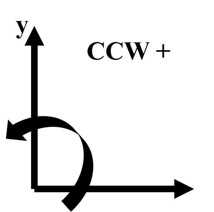
Figure \(\PageIndex{1}\): Coordinate System for Statics.
Critical Idealizations/Assumptions in Statics Problems:
There are several critical assumptions/idealization that we will utilize when working on statics problems specifically that
• Particle Assumption: Particle has mass but we will effectively ignore the geometry of a particle
• Rigid Body Assumption: The body will behave rigid, meaning that when a force is applied there will be no deformation, either elastic or plastic, of that body. Therefore the material properties of the body do not exist.
• Concentrated Force Assumption: The force will be concentrated and localized at a single point
Force As a Vector or First Rank Tensor Property
![]()
Force is not a scalar property it is in fact a vector quantity, meaning force has both direction and magnitude. Many will also refer to force as a first rank tensor property as well. Let’s look at some examples of vectors as a concept first as seen in Fig.2.
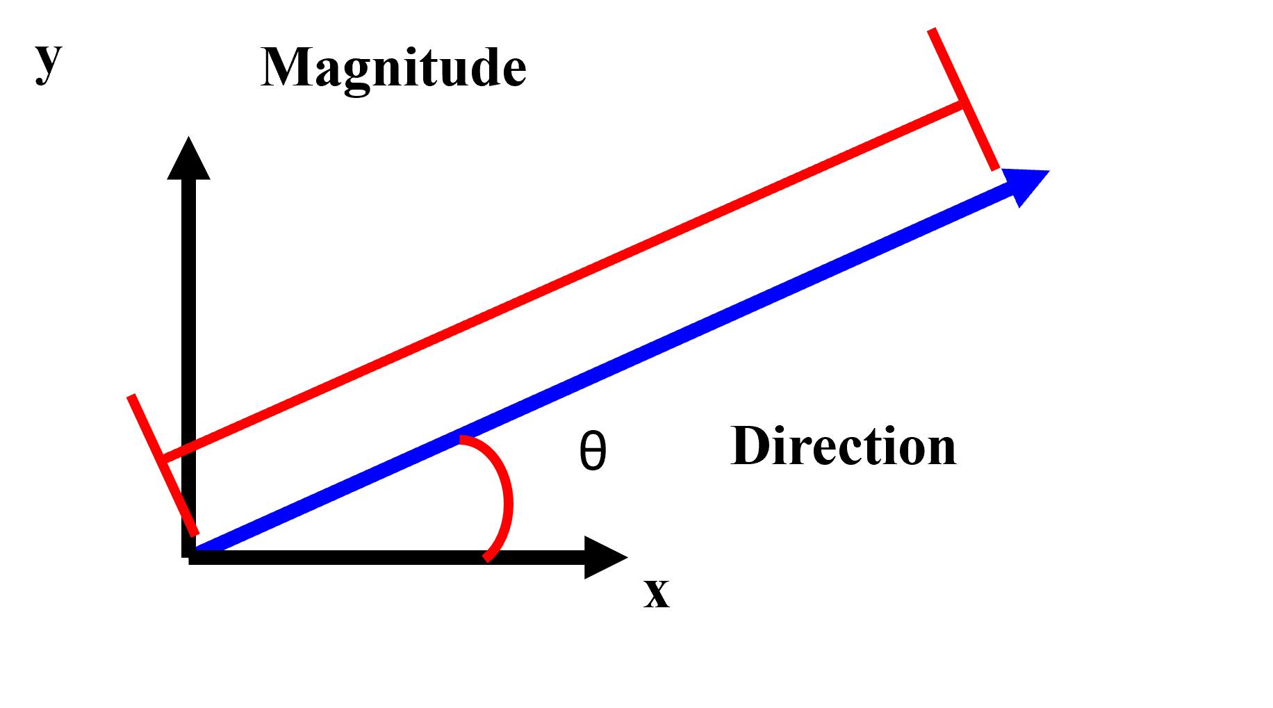
Figure \(\PageIndex{2}\): Force as a vector/first rank tensor property.
This force can also be resolved into x and y components specifically
\[F = F_x i + F_y j\]
where Fx and Fy are respective magnitudes of the force components in the x and y and i and j are Cartesian vector notation. This can be seen in Fig.3
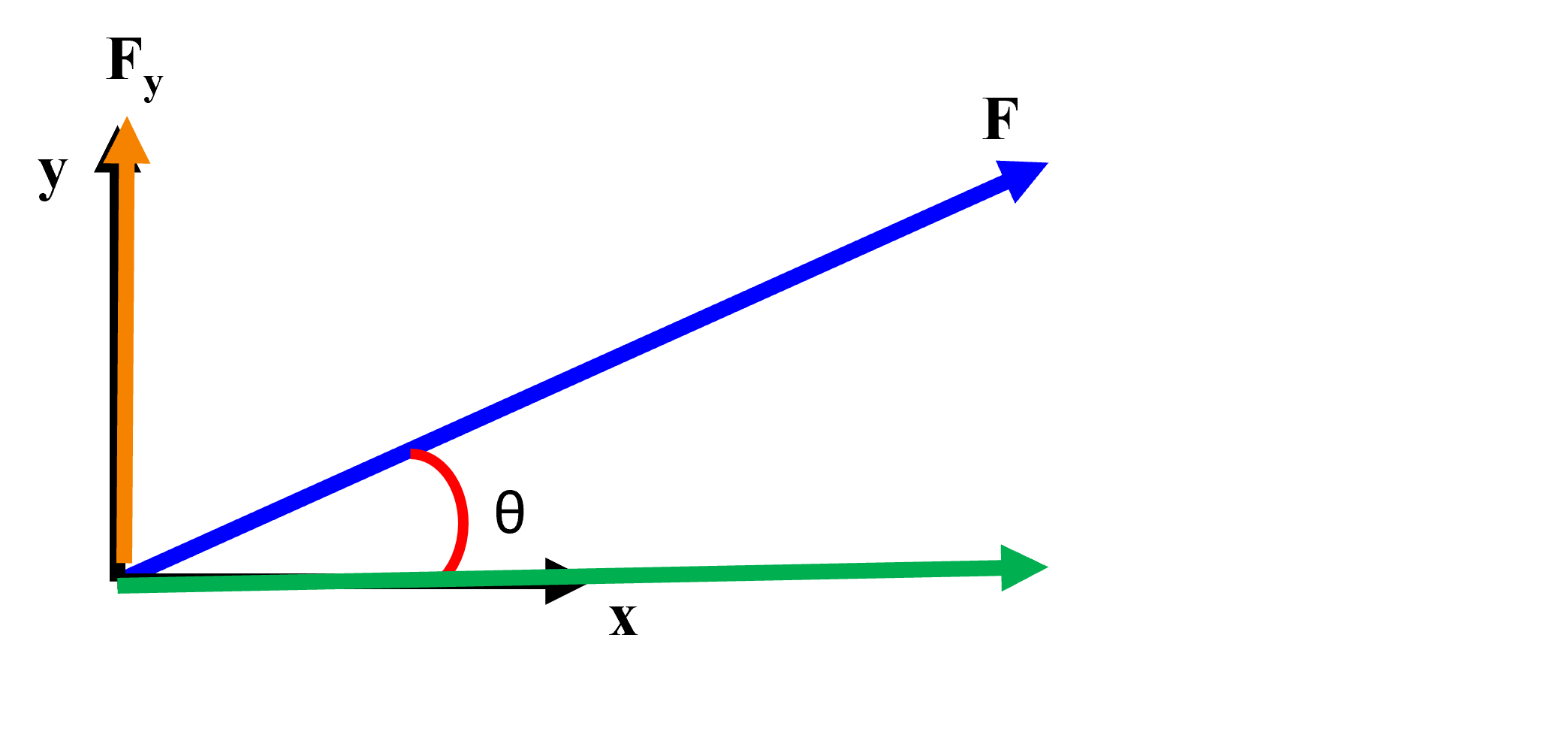
Figure \(\PageIndex{3}\): Force Components.
Additionally as we have the angle, θ we can also define that
\[\begin{align} F_x = F \cos \theta\\ F_y = F \sin \theta \end{align}\]
We can do an example together and find what is the resultant force in the x and y directions which can be defined as
\[\begin{align} F_{R_x} = \sum F_x\\ F_{R_y} = \sum F_y \end{align}\]
Here we can see an example below in Fig.4
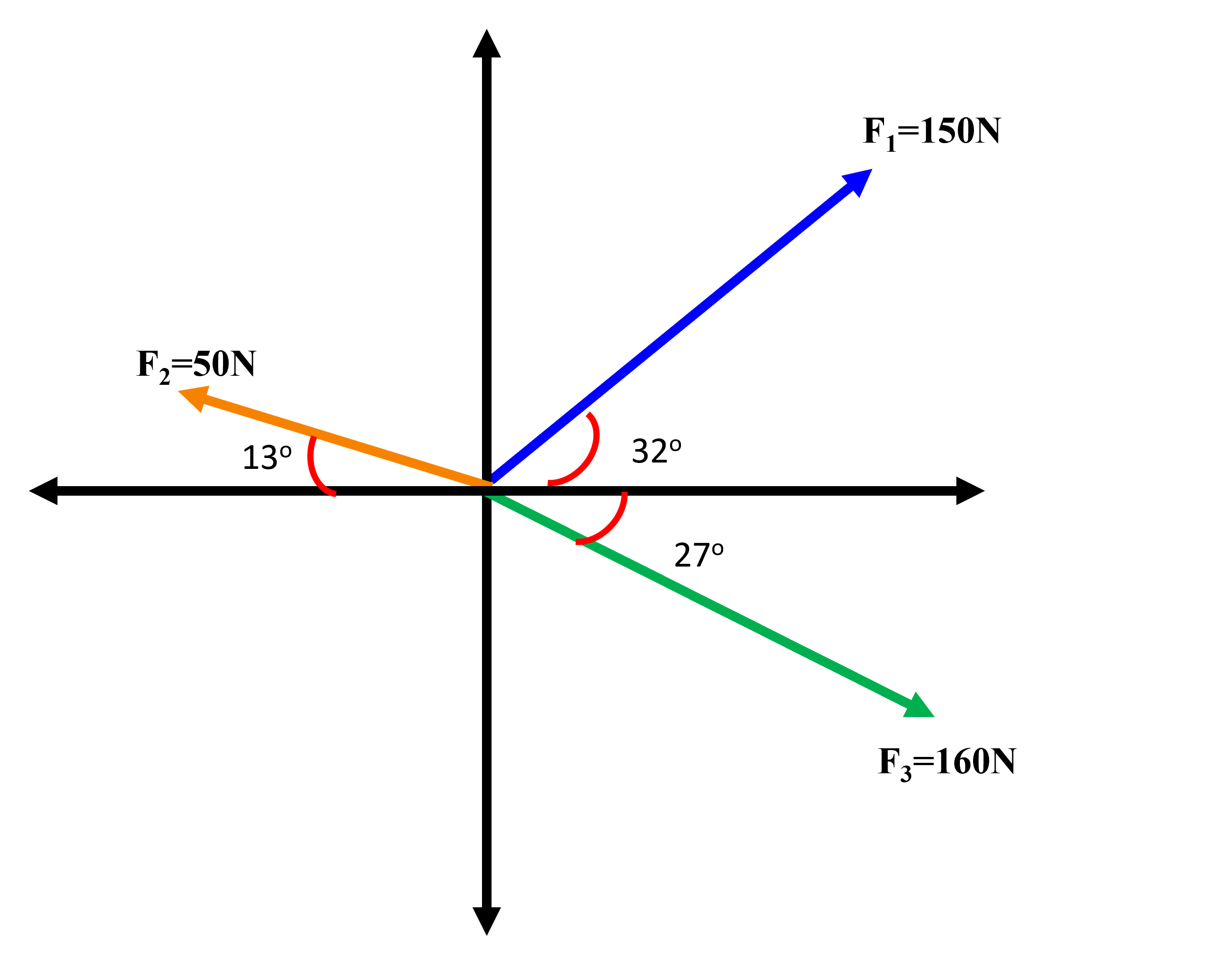
Figure \(\PageIndex{4}\): Force Summation Example.
Sum of Forces Must Be Equal to Zero
We can also apply static equilibrium conditions and Newton’s First law to solve for the two unknown forces, F1 and F2, as seen in Fig.5.

Figure \(\PageIndex{5}\): Sum of forces must be zero.
Moment
A moment is defined as
\[M_o = Fd\]
where F is the magnitude of force and d is the perpendicular distance from the origin, o, to the line of action of the force as seen below in Fig.6

Figure \(\PageIndex{6}\): Moments.
Spring Force
We will often come across springs in mechanical engineering and use springs as idealizations for some elements of mechanical designs and systems. A spring force can be defined as
\[F =k \Delta x\]
where k is a spring constant and \(\Delta\) is the change in length of a spring this is also seen in Fig.7
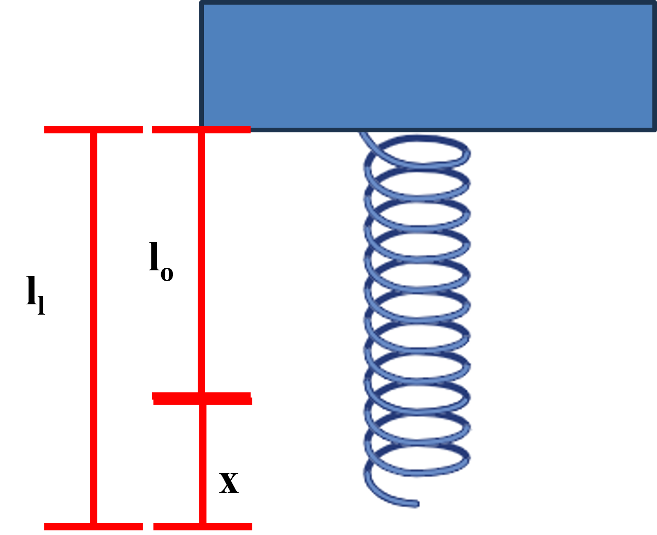
Figure \(\PageIndex{7}\): Spring Force.
Additionally if you have a mass attached to a cable/pulley/wire you will have tension in the wire, T, and the mass will have a weight, W = mg which you can see in
Fig.8
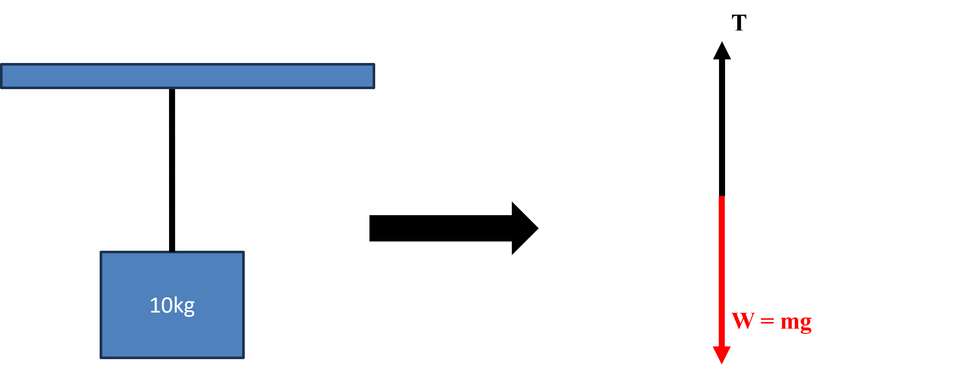
Figure \(\PageIndex{8}\): Tension in wire and weight.
Static Equilibrium Practice Problem!!
To solve this problem let’s perform our statics problem solving algorithm.
(1) Idealize Real System
(2) Define Coordinate system
(3) Draw Free Body Diagram (FBD)
(4) Write Equilibrium Expressions
(5) Solve for Unknowns
Consider the situation of a person with a mass of 100kg on a scaffold which is suspended via two cables as seen in Fig.9
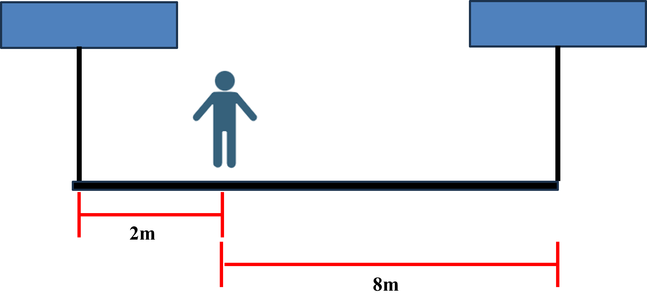
Figure \(\PageIndex{9}\): Person on a scaffold problem.
So in this real system we are going to make several idealizations the biggest being that we will neglect the mass of the scaffold itself and we will ignore friction in this scenario as well. Additionally, we will assume the scaffold is rigid and therefore will not deform in this system.
We have defined our coordinate system in this diagram and now we will draw our Free Body Diagram. To do so we will free the body which has forces exerted on it, i.e. the scaffold. So we will draw the scaffold and free this body from the surroundings and replace the surroundings by idealizing them as forces which can be seen in Fig.10
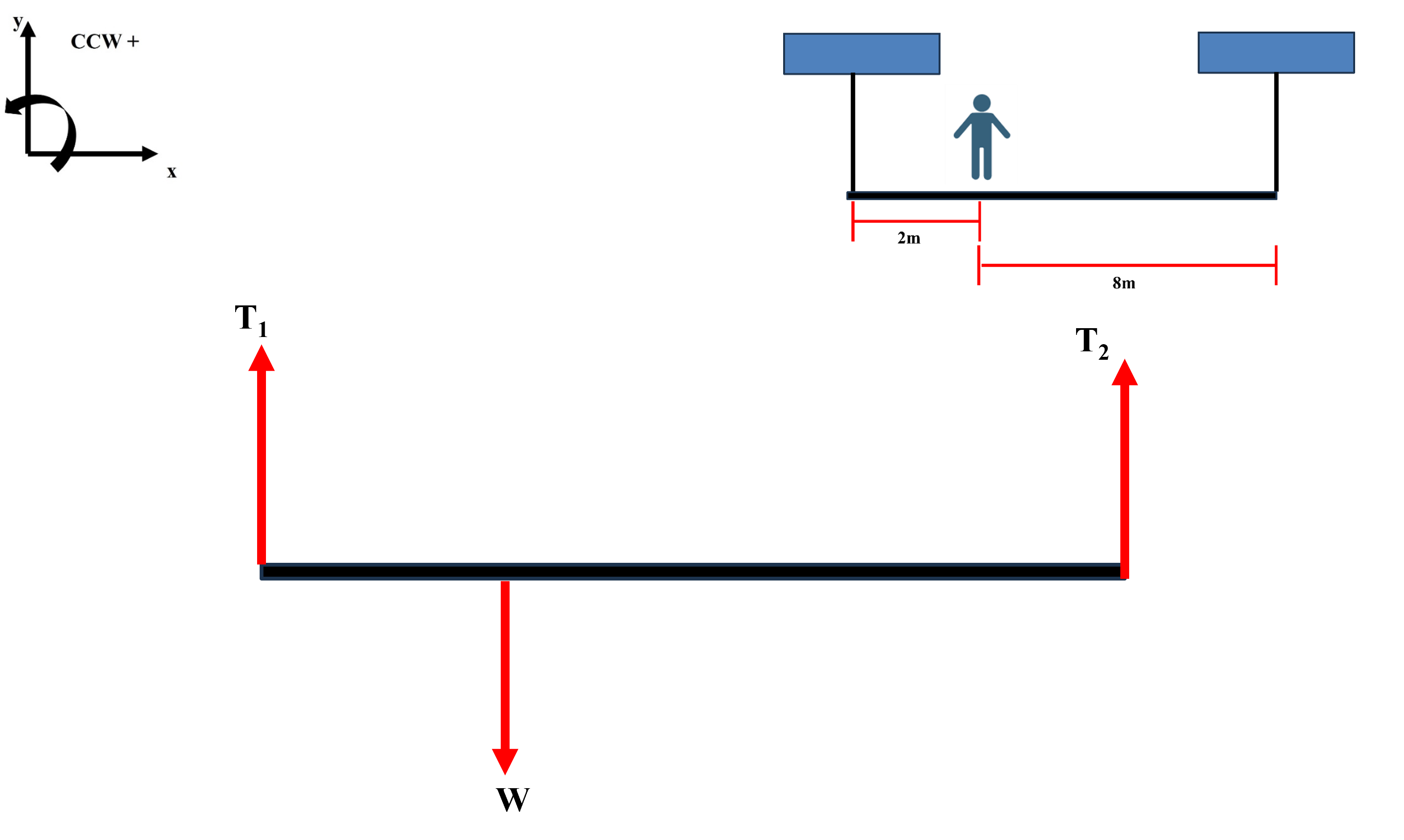
Figure \(\PageIndex{10}\): Free Body Diagram.
We can now write out our fundamental equations which are the sum of the moments and the sum of the forces must be equal to zero if we are indeed in static equilibrium.
Let us first consider the x-direction and even though we have no forces we can still write out that
\[\sum F_x = 0\]
and this will hold true.
Now we can consider forces in the y-direction and we have that
\[\sum F_y = 0 = -W +T_1+T_2\]
where we know that W = mg and we know that the mass of the person is 100kg.
Now we can write the sum of the moments about any origin will be zero and I will choose the origin to be located at T1 so
\[\sum M_{T_1} = 0 = -W \cdot 2m + T_2 \cdot 10m\]
So we have two equations and two unknowns and now we can solve the problem for the unknowns!
Let’s consider another problem this time a SeeSaw!
SeeSaw
To solve this problem let’s perform our statics problem solving algorithm.
(1) Idealize Real System
(2) Define Coordinate system
(3) Draw Free Body Diagram (FBD)
(4) Write Equilibrium Expressions
(5) Solve for Unknowns
Consider the situation of a person, P1 with a mass of 100kg on a SeeSaw and find all the resulting forces to keep the SeeSaw flat as seen in Fig.11
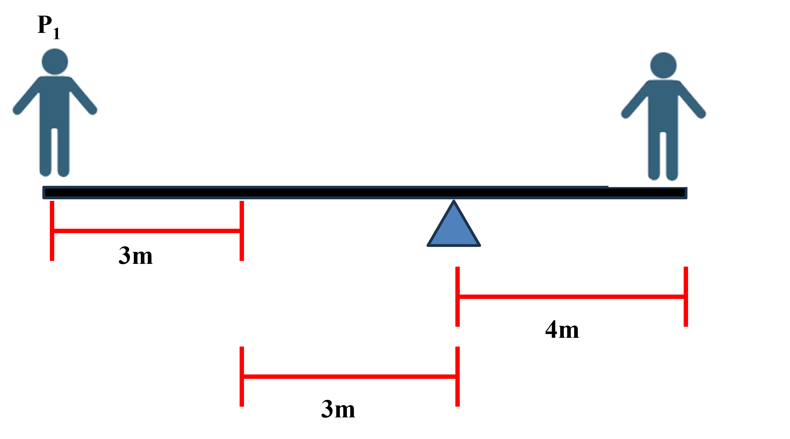
Figure \(\PageIndex{11}\): SeeSaw.
So in this real system we are going to make several idealizations the biggest being that we will neglect the mass of the SeeSaw itself. Additionally, we will assume the SeeSaw is rigid and therefore will not deform in this system.
We have defined our coordinate system in this diagram and now we will draw our Free Body Diagram. To do so we will free the body which has forces exerted on it, i.e. the SeeSaw. So we will draw the SeeSaw and free this body from the surroundings and replace the surroundings by idealizing them as forces which can be seen in Fig.12
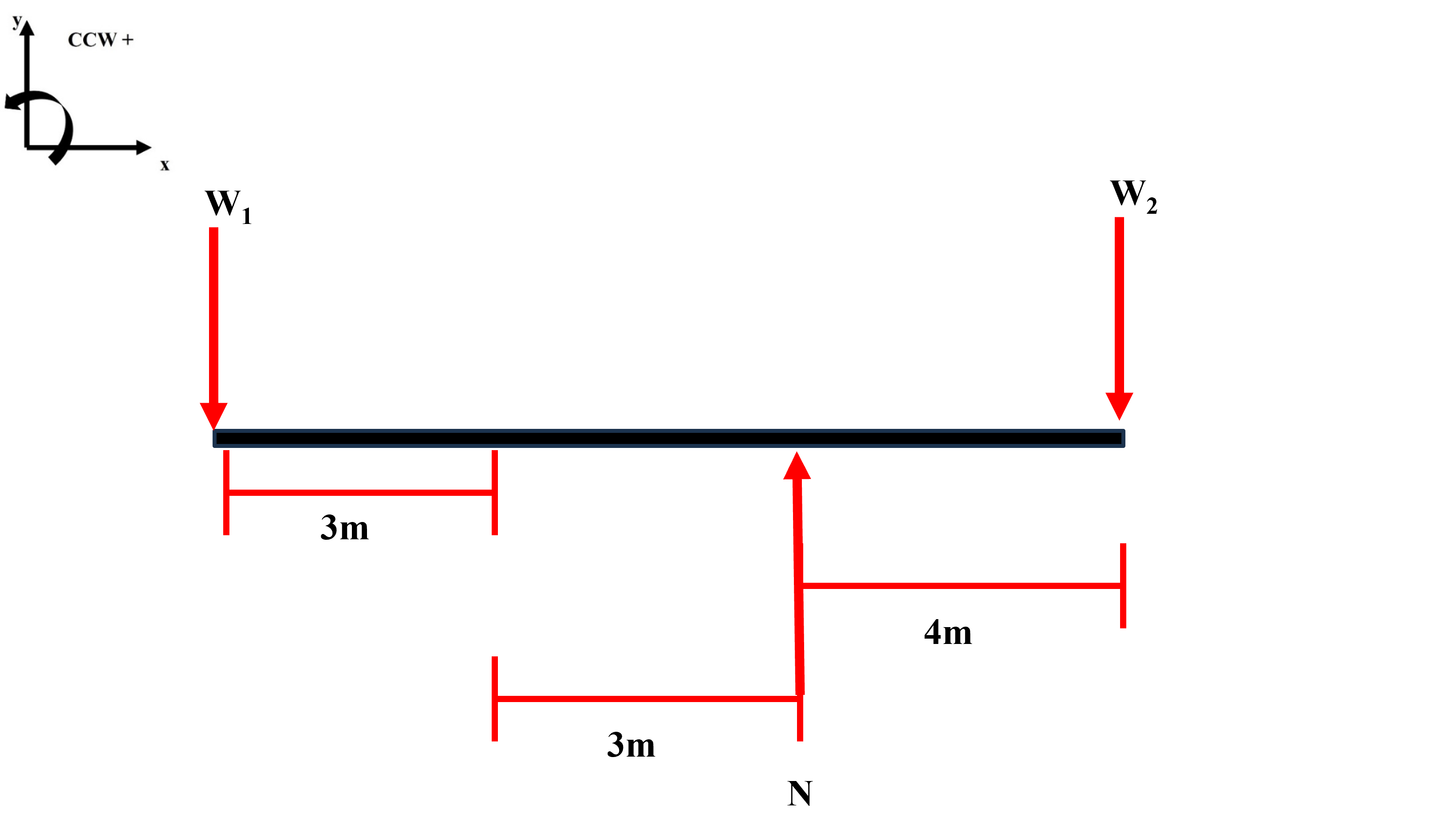
Figure \(\PageIndex{12}\): Free Body Diagram.
We can now write out our fundamental equations which are the sum of the moments and the sum of the forces must be equal to zero if we are indeed in static equilibrium.
Let us first consider the x-direction and even though we have no forces we can still write out that
\[\sum F_x = 0\]
and this will hold true.
Now we can consider forces in the y-direction and we have that
\[\sum F_y = 0 = -W_1 +N -W_2\]
where we know that W1 = mg and we know that the mass of the person is 100kg.
Now we can write the sum of the moments about any origin will be zero and I will choose the origin to be located at W1 so
\[\sum M_{W_1} = 0 = N \cdot 6m - W_2 \cdot 10m\]
So we have two equations and two unknowns and now we can solve the problem for the unknowns!
Types of Friction:
In this lecture we will predominantly discuss friction in the context of dry friction or Coloumb friction which occurs between contacting surfaces of bodies when there is no lubricating fluids.
One of the important things to note when considering dry friction is that the friction force F may not be enough to balance the applied force P when the surface is slippery. In fact the value of the frictional force increases as P increases until reaching a maximum value of limit of static frictional force, Fs, which is defined as
\[F_s = \mu_s N\]
where µs is the coefficient of static friction and we see that the limiting static frictional force is directly proportional to the resultatn normal. You can also see that friction will oppose the direction of impending motion and is tangent to the contacting surface. Once the magnitude of P becomes larger than Fs the friction decreases to a smaller value Fk which is the kinetic frictional force defined as
\[F_k = \mu_k N\]
and this can be seen here

Figure \(\PageIndex{13}\): Dry Friction: Force is lower than limit of static friction.

Figure \(\PageIndex{14}\): Dry Friction: Force is close than limit of static friction.
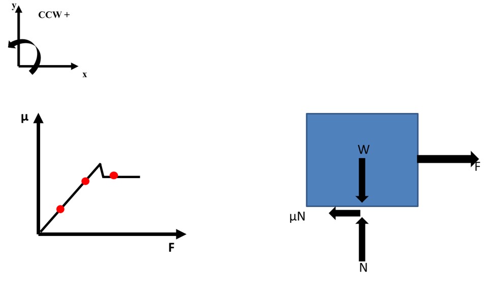
Figure \(\PageIndex{15}\): Dry Friction: Force is larger than limit of static friction and friction force decreases to limit of kinetic friction.
Typically, when dealing with dry friction you will encounter problems where there will friction that occurs even without any apparent impending motion, impending motion at all points of contact, or impending motion at certain points contact. However, you will still utilize the same problem solving algorithm that we will introduce shortly.
You may also friction when using wedges to adjust the elevation of parts, frictional forces on screws, flat belts, bearings, and rolling resistance as well all of which can be summarized in the figure below however again for this particular lecture we will focus primarily on dry friction.
Tire Blowout 0.7 Miles From ATI Plant in Louisville, Ohio
I worked for a while in Pittsburgh at ATI in the metallurgy industry. Part of the job required driving to a plant in the middle of the night to Louisville, Ohio, a plant in a very small town that is isolated. During my first year I was driving at 3AM in January and only 0.7 miles from the plant my tire ruptured and isolated, alone, I had to pull the car (finally getting to utilize my emergency rope kit) 0.7 long cold miles to the plant. Why didn’t I drive might you ask, well I was worried about damaging the tire, it was cold and I was extremely frazzled and tired from the experience.
The Jeep has mass of approximately 1600kg and it is quite cold and slick so the coefficient of friction between the tires and the substrate is approximately µs = 0.3 and the front tires were free to rotate but the back tires are locked. I can exert a force of approximately 3000N will the car move?
I exert a force on the cable of approximately 3000N. Considering the mass of the car is 1600kg and the coefficient of friction between the tire and the surface is µs = 0.3. Will the car move?
To solve this problem let’s perform our statics problem solving algorithm.
(1) Idealize Real System
(2) Coordinate system
(3) Free Body Diagram
(4) Write Equilibrium Expressions
(5) Solve for Unknowns
So we can do the following steps and first idealize the system as seen here.

Figure \(\PageIndex{16}\): Idealized System of Pulling Car.
Then we define our coordinate system and can simultaneously draw our free body diagram.

Figure \(\PageIndex{17}\): Free Body Diagram.
The important thing to note here is the determination of the direction of the frictional force. The friction force must be tangent to the contact surface and should oppose the direction of impending motion.
With the FBD complete we can now write out our systems of equilibrium expressions \[\begin{align} \Sigma F_x = 0 = -T\cos(\theta) + \mu_s N_2\\ \Sigma F_y = 0= T \sin(\theta)+N_1+N_2-W\\ \Sigma M_C = 0 = (4 ft)W - (9 ft)N_1 + (1 ft) T\cos(\theta) - (10.6 ft)T\sin(\theta) \end{align}\]
But the car didn’t move funnily enough, I suspect that both brakes are locked. Well let’s repeat our process and we already have our idealization. Now we can define the coordinate system and free the body.
Now let’s write out our systems of equations \[\begin{align} \Sigma F_x = 0 = -T\cos(\theta) + \mu_s N_2+\mu_s N_1\\ \Sigma F_y = 0= T \sin(\theta)+N_1+N_2-W\\ \Sigma M_C = 0 = (4 ft)W - (9 ft)N_1 + (1 ft) T\cos(\theta) - (10.6 ft)T\sin(\theta) \end{align}\]

Figure \(\PageIndex{18}\): Free Body Diagram.
Person on a Ladder
Recently I had to take down my holiday lights and this was after cleaning the gutters but before I have to go up on the remove to spray moss remover, so much work to do!!!
Anyway, when I am up on the ladder and lean it against the wall of the house I can feel the difference in friction between the wall and the ground. Now I am using a 4m tall ladder and my mass is approximately 100kg (after a workout).... and the angle is approximately 18o. The wall is stucco and in contact with the steel ladder the coefficient of friction with that surface is approximately µ1 = 0.7. What coefficient of friction is required on the ground to prevent the ladder from moving? Is the ladder likely to fall? Do I have to lose weight??
Considering that I have a mass of 100kg we can neglect the mass and weight of the ladder. What is the coefficient of friction, µs,2 required to prevent the ladder from slipping?
Now let’s start with our problem solving algorithm and start to idealize the system as seen here.

Figure \(\PageIndex{19}\): Idealization of me cleaning gutters.
Now let’s define our coordinate system and free the body

Figure \(\PageIndex{20}\): Free Body Diagram.
Finally, let’s write out our equilibrium expressions and solve \[\begin{align} \Sigma F_x = 0 = N_1 - \mu_{s,2} N_2\\ \Sigma F_y = 0 = \mu_{s,1} N_1 - W +N_2\\ \Sigma M_{o} = 0 = (1.8 m) W - (4 \sin(\theta) m) N_1 - (4 \cos(\theta) m) \mu_{s,1} N_1 \end{align} \]

