
Chapter 3: Dynamics and Vibrations
- Page ID
- 107042
\( \newcommand{\vecs}[1]{\overset { \scriptstyle \rightharpoonup} {\mathbf{#1}} } \)
\( \newcommand{\vecd}[1]{\overset{-\!-\!\rightharpoonup}{\vphantom{a}\smash {#1}}} \)
\( \newcommand{\dsum}{\displaystyle\sum\limits} \)
\( \newcommand{\dint}{\displaystyle\int\limits} \)
\( \newcommand{\dlim}{\displaystyle\lim\limits} \)
\( \newcommand{\id}{\mathrm{id}}\) \( \newcommand{\Span}{\mathrm{span}}\)
( \newcommand{\kernel}{\mathrm{null}\,}\) \( \newcommand{\range}{\mathrm{range}\,}\)
\( \newcommand{\RealPart}{\mathrm{Re}}\) \( \newcommand{\ImaginaryPart}{\mathrm{Im}}\)
\( \newcommand{\Argument}{\mathrm{Arg}}\) \( \newcommand{\norm}[1]{\| #1 \|}\)
\( \newcommand{\inner}[2]{\langle #1, #2 \rangle}\)
\( \newcommand{\Span}{\mathrm{span}}\)
\( \newcommand{\id}{\mathrm{id}}\)
\( \newcommand{\Span}{\mathrm{span}}\)
\( \newcommand{\kernel}{\mathrm{null}\,}\)
\( \newcommand{\range}{\mathrm{range}\,}\)
\( \newcommand{\RealPart}{\mathrm{Re}}\)
\( \newcommand{\ImaginaryPart}{\mathrm{Im}}\)
\( \newcommand{\Argument}{\mathrm{Arg}}\)
\( \newcommand{\norm}[1]{\| #1 \|}\)
\( \newcommand{\inner}[2]{\langle #1, #2 \rangle}\)
\( \newcommand{\Span}{\mathrm{span}}\) \( \newcommand{\AA}{\unicode[.8,0]{x212B}}\)
\( \newcommand{\vectorA}[1]{\vec{#1}} % arrow\)
\( \newcommand{\vectorAt}[1]{\vec{\text{#1}}} % arrow\)
\( \newcommand{\vectorB}[1]{\overset { \scriptstyle \rightharpoonup} {\mathbf{#1}} } \)
\( \newcommand{\vectorC}[1]{\textbf{#1}} \)
\( \newcommand{\vectorD}[1]{\overrightarrow{#1}} \)
\( \newcommand{\vectorDt}[1]{\overrightarrow{\text{#1}}} \)
\( \newcommand{\vectE}[1]{\overset{-\!-\!\rightharpoonup}{\vphantom{a}\smash{\mathbf {#1}}}} \)
\( \newcommand{\vecs}[1]{\overset { \scriptstyle \rightharpoonup} {\mathbf{#1}} } \)
\(\newcommand{\longvect}{\overrightarrow}\)
\( \newcommand{\vecd}[1]{\overset{-\!-\!\rightharpoonup}{\vphantom{a}\smash {#1}}} \)
\(\newcommand{\avec}{\mathbf a}\) \(\newcommand{\bvec}{\mathbf b}\) \(\newcommand{\cvec}{\mathbf c}\) \(\newcommand{\dvec}{\mathbf d}\) \(\newcommand{\dtil}{\widetilde{\mathbf d}}\) \(\newcommand{\evec}{\mathbf e}\) \(\newcommand{\fvec}{\mathbf f}\) \(\newcommand{\nvec}{\mathbf n}\) \(\newcommand{\pvec}{\mathbf p}\) \(\newcommand{\qvec}{\mathbf q}\) \(\newcommand{\svec}{\mathbf s}\) \(\newcommand{\tvec}{\mathbf t}\) \(\newcommand{\uvec}{\mathbf u}\) \(\newcommand{\vvec}{\mathbf v}\) \(\newcommand{\wvec}{\mathbf w}\) \(\newcommand{\xvec}{\mathbf x}\) \(\newcommand{\yvec}{\mathbf y}\) \(\newcommand{\zvec}{\mathbf z}\) \(\newcommand{\rvec}{\mathbf r}\) \(\newcommand{\mvec}{\mathbf m}\) \(\newcommand{\zerovec}{\mathbf 0}\) \(\newcommand{\onevec}{\mathbf 1}\) \(\newcommand{\real}{\mathbb R}\) \(\newcommand{\twovec}[2]{\left[\begin{array}{r}#1 \\ #2 \end{array}\right]}\) \(\newcommand{\ctwovec}[2]{\left[\begin{array}{c}#1 \\ #2 \end{array}\right]}\) \(\newcommand{\threevec}[3]{\left[\begin{array}{r}#1 \\ #2 \\ #3 \end{array}\right]}\) \(\newcommand{\cthreevec}[3]{\left[\begin{array}{c}#1 \\ #2 \\ #3 \end{array}\right]}\) \(\newcommand{\fourvec}[4]{\left[\begin{array}{r}#1 \\ #2 \\ #3 \\ #4 \end{array}\right]}\) \(\newcommand{\cfourvec}[4]{\left[\begin{array}{c}#1 \\ #2 \\ #3 \\ #4 \end{array}\right]}\) \(\newcommand{\fivevec}[5]{\left[\begin{array}{r}#1 \\ #2 \\ #3 \\ #4 \\ #5 \\ \end{array}\right]}\) \(\newcommand{\cfivevec}[5]{\left[\begin{array}{c}#1 \\ #2 \\ #3 \\ #4 \\ #5 \\ \end{array}\right]}\) \(\newcommand{\mattwo}[4]{\left[\begin{array}{rr}#1 \amp #2 \\ #3 \amp #4 \\ \end{array}\right]}\) \(\newcommand{\laspan}[1]{\text{Span}\{#1\}}\) \(\newcommand{\bcal}{\cal B}\) \(\newcommand{\ccal}{\cal C}\) \(\newcommand{\scal}{\cal S}\) \(\newcommand{\wcal}{\cal W}\) \(\newcommand{\ecal}{\cal E}\) \(\newcommand{\coords}[2]{\left\{#1\right\}_{#2}}\) \(\newcommand{\gray}[1]{\color{gray}{#1}}\) \(\newcommand{\lgray}[1]{\color{lightgray}{#1}}\) \(\newcommand{\rank}{\operatorname{rank}}\) \(\newcommand{\row}{\text{Row}}\) \(\newcommand{\col}{\text{Col}}\) \(\renewcommand{\row}{\text{Row}}\) \(\newcommand{\nul}{\text{Nul}}\) \(\newcommand{\var}{\text{Var}}\) \(\newcommand{\corr}{\text{corr}}\) \(\newcommand{\len}[1]{\left|#1\right|}\) \(\newcommand{\bbar}{\overline{\bvec}}\) \(\newcommand{\bhat}{\widehat{\bvec}}\) \(\newcommand{\bperp}{\bvec^\perp}\) \(\newcommand{\xhat}{\widehat{\xvec}}\) \(\newcommand{\vhat}{\widehat{\vvec}}\) \(\newcommand{\uhat}{\widehat{\uvec}}\) \(\newcommand{\what}{\widehat{\wvec}}\) \(\newcommand{\Sighat}{\widehat{\Sigma}}\) \(\newcommand{\lt}{<}\) \(\newcommand{\gt}{>}\) \(\newcommand{\amp}{&}\) \(\definecolor{fillinmathshade}{gray}{0.9}\)Pre-recorded videos covering these topics can be found in the YouTube playlist here: https://www.youtube.com/playlist?lis...13bhGLLZBQkZhd.
Now that we have the fundamentals of Statics we can start to analyze dynamic systems and we will start to work with Newton’s 2nd Law as seen below.
Newtons Laws
• Newton’s 1st Law: If a body is at rest or moving at a constant velocity in a straight line it will remain at rest or keep moving in a straight line at constant velocity unless acted upon by a force.
• Newton’s 2nd Law:
\[F = ma\]
• Newton’s 3rd Law: When two bodies interact they apply forces to one another that are equal in magnitude but opposite in direction, i.e. the law of action and reaction.
For Statics, the 1st and 3rd laws are of critical importance. Dynamics deals with Newton’s 2nd law so we will investigate that further in this class. Furthermore, we can make some simplifications to Newton’s 1st law and simply re-rewrite it as follows \[\begin{align} \Sigma F =0\\ \Sigma M =0 \end{align}\]
This is how we will interpret this first law and the third law.
Fundamentals of Dynamics
Before we begin to tackle problems it is important to define some critical parameters and terms when it comes to dynamics. We will typically be analyzing the displacement of a system/body and we will define the position of a body as \[x(t)\]
The position is a function of time and the velocity can be defined as \[\begin{align} v = \frac{dx}{dt} \end{align} \]
and very importantly the acceleration is defined as \[\begin{align} a = \frac{dv}{dt} = \frac{d^2 x}{dt^2} \end{align}\]
These definitions all refer to Translational Motion and the fundamental equation that governs translation motion is Newton’s 2nd law that \[\begin{align} \sum F = ma \end{align}\]
We can also say that for translation that \[\begin{align}\sum M_G = 0 \end{align}\]
so the sum of the moments about the center of mass will be 0 for a body undergoing translation but you can also solve for the moment about any point P and use the following expression \[\begin{align} \sum M_P = \sum \bigg(M_k\bigg)_P \end{align}\]
We will also encounter Rotational Motion as well and rotational motion occurs when a body rotates around a fixed axis and they body will change the angular position and we will track the angular displacement as defined below \[\begin{align} \theta (t) \end{align}\]
The angular velocity can be defined as \[\begin{align} \omega = \frac{d\theta}{dt} \end{align}\]
and angular acceleration can be defined as \[\begin{align}\alpha = \frac{d\omega}{dt} = \frac{d^2 \theta}{dt^2} \end{align}\]
It is also important to note that in terms of angular acceleration you will typically encounter a normal and tangential component which can be defined as \[\begin{align} a_t = \alpha r\\ a_n = \omega^2 r \end{align}\]
and rotational motion is governed by the fundamental equation that \[\begin{align} \sum M_G = I_G \alpha \end{align}\]
So the fundamental equations of dynamics will be \[\begin{align} \sum F_x = ma\\ \sum F_y = ma\\ \sum M_G = I_G \alpha\\ \end{align}\]
or more generally around some point P .
Problem Solving Dynamics Algorithm
We will follow a similar problem solving algorithm to the one that we performed in
To solve this problem let’s perform our dynamics problem solving algorithm.
(1) Idealize Real System
(2) Coordinate System
(3) Free Body Diagram
(4) Kinetic Diagram
(5) Write Equilibrium Expressions
(6) Solve for Unknowns
The key distinction here is the drawing of a kinetic body diagram so now lets start to solve some problems together!
Truck Carrying Load
Let’s consider the following problem of a 100kg table on a truck bed that is accelerating. The static coefficient of friction between the legs of the table and the truck bed is µs = 0.3. We want to solve for the maximum acceleration of the truck without causing the assembly to move relative to the truck as well as the reaction forces at A and B. The center of the mass of the table is indicated at G.
To solve this problem let’s perform our dynamics problem solving algorithm.
(1) Idealize Real System
(2) Coordinate System
(3) Free Body Diagram
(4) Kinetic Diagram
(5) Write Equilibrium Expressions
(6) Solve for Unknowns
We will have to make several idealizations in this problem specifically we will ignore any air resistance and that the truck will move at a constant acceleration as seen in Fig.1

Figure \(\PageIndex{1}\): Table on a Truck Bed.
We can then define our coordinate system and draw our free body diagram (FBD)
of our body which is the table in Fig.2
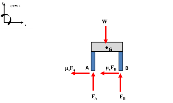
Figure \(\PageIndex{2}\): Free Body Diagram
We can also draw our kinetic diagram (KD) for the body as well in table Fig.3

Figure \(\PageIndex{3}\): Kinetic Body Diagram
We can now write out our fundamental equations and let’s start out looking at translation first and in the x-direction and because we want it to not move relative to the truck acceleration it must have the same acceleration\[\begin{align}\sum F_x = ma_x = -\mu_s F_A - \mu_s F_B \end{align}\]
We can also write out for translation in the y-direction where there is no acceleration\[\begin{align}\sum F_y = 0 = -W +F_A +F_B\end{align}\]
Finally we can use the relationship for the sum of the moments about the center of mass to write\[\begin{align}\sum M_G = 0 = -\mu_s F_A 0.6 - \mu_s F_B 0.6 - F_A 0.15 +F_B 0.15 \end{align}\]
So we have three equations and three unknowns and now we can solve the problem for the unknowns!
Frisbee Problem
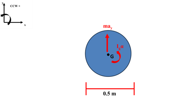
Let’s make a Frisbee launcher to launch a 0.5m diameter with a mass of 0.05kg and when
it is ejected we want a linear acceleration of 10\(\frac{m}{s^2}\) and an angular acceleration of 20 \(\frac{rad}{s^2}\). Solve for the values of \(F_1\) and \(F_2\) to meet these criteria. Ignore friction between the Frisbee and launching pads. Additionally the \(I_G = \frac{m r^2}{2}\) for a think disk through axis perpendicular to the face of the Frisbee.
To solve this problem let’s perform our dynamics problem solving algorithm.
(1) Idealize Real System
(2) Coordinate System
(3) Free Body Diagram
(4) Kinetic Diagram
(5) Write Equilibrium Expressions
(6) Solve for Unknowns
We can then define our coordinate system and draw our free body diagram (FBD) of our body which is the Frisbee in Fig.4

We can also draw our kinetic diagram (KD) for the body as well in Fig.5
We can now write out our fundamental equations and let’s start out looking at translations first and in the x-direction and in this direction we have no translational acceleration \[\begin{align}\sum F_x = 0\end{align}\]
We can also write out for translation in the y-direction where there is acceleration\[\begin{align}\sum F_y = ma_y = F_1+F_2 \end{align}\]
We can also use the relationship that we have for moments about a point and we will choose the location at 1 so \[\begin{align}\sum M_1 = 2 r F_2 = I_G \alpha + r m a_y \end{align}\]
So we have two equations and two unknowns and now we can solve the problem for the unknowns!
Vibrations
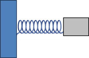
We will often encounter systems that are vibrating and vibrations are the oscillating motion of a body or system from a position of equilibrium. There are many types of vibrations but to give an introduction to concept of vibrations we will consider the oscillation of a mass connected to a spring that is also connected to a wall as seen in Fig.6
We can then draw our FBD in Fig.7

We can then draw our KBD in Fig.8

We can solve this problem like we have done similarly and define our critical equations of motion and we see that\[\begin{align} \sum F_y = 0 = -mg + N\end{align}\]
and the acceleration in the y-direction is zero because there is no motion/vibration in that direction and we can similarly analyze the motion in the x-direction \[\begin{align}\sum F_x = ma = -kx\end{align}\]
We can also re-write this as a time derivative\[\begin{align}a = \frac{d^2x}{dt^2} = \ddot{x}\end{align}\]
So the equation then becomes \[\begin{align}m \ddot{x} +k x = 0\end{align}\]
or we can define a natural frequency, \(\omega_n = \sqrt{\frac{k}{m}}\), and re-write \[\begin{align}\ddot{x} + \omega^2 x =0\end{align}\]
This is an example of a second order ordinary differential equation because we have a function of position, x, as a function of time and it is second order because we are dealing with a second derivative. If we can solve this problem by defining two initial conditions to solve the general solution that will have the form of \[\begin{align} x(t) = A \sin \omega_n t + B \cos \omega_n t \end{align}\]
This type of motion an example of a motion termed simple harmonic motion and you will do a fun lab to confirm the natural frequency of a system.