Chapter 4: Materials Science and Engineering

Sign Conventions:

To begin let’s talk about units and sign conventions. We will define any forces, stresses, or strain in tension as positive and any forces, stresses, or strain under compression will be considered negative. Additionally we will consider moments that are counter clockwise as positive and clockwise as negative.

Stress-Strain Curve:

When a material is placed under a stress state we will typically plot a stress-strain curve and that curve typically will have 3 distinct regions: I) Elastic, II) Plastic, III) Fracture.

I) Elastic Regime:

In the elastic regime the stress strain response is linear and defined by the expression below which should be familiar (Hooke’s Law) \begin{align} \sigma = E\epsilon \end{align}

where E, sometimes Y, is defined as the Young’s Modulus. It describes the stiffness of the material and is a material constant. Metals are typically in the 100s of GPa, ceramics are high 200’s and 300’s of GPa, polymers are closer to on the order of 1 GPa. In the elastic region the strain is completely reversible, i.e. there is no permanent or plastic deformation. You are just pulling on the bonds not breaking any bonds.

II) Plastic Regime:

Here you are plastically deforming the material and this is signified microstructurally by the breaking of bonds and the movement of dislocations. Additionally with plastic dislocation the strain is not reversible, if you remove the force the strain remains. It is signified to begin on the stress strain curve by σ_y which is the yield stress and ϵ_y the yield strain. The σ_UTS is the ultimate tensile strength and it denotes the onset of necking which is where the instantaneous area is now smaller than the original area.

III) Fracture:

As the name denotes this is where the material catastrophically fractures and is denoted by σ_f which is the fracture stress and the ϵ_f is the fracture strain[?].

At this point we need to stop and make a clear point about the language that we have to use when discussing the material properties of materials. Word choice is critical here because they mean very different things. When we talk about the stiffness of materials we are talking about the Young’s modulus of the material. The higher the Young’s modulus the stiffer the material. When we talk about strength we are talking about the yield strength, the ultimate tensile strength, or the fracture stress or strength. We we are talking about how ductile a material is we are talking about the strain at failure. We also often talk about material resilience and toughness as well.

We define elastic strain energy (ESE) which is defined as \begin{align}U_{ESE} = V \int^{\epsilon_{y}}_{0}\sigma_{11} d\epsilon_{11}\end{align}

where V is the volume which gives us units of energy. This is the blue shaded portion. Toughness is defined as\begin{align}U_{T} = V \int^{\epsilon_{f}}_{0}\sigma_{11} d\epsilon_{11}\end{align}

If a material is not as stiff it is called compliant, if a material is not strong it is weak, and if a material is not tough it is termed brittle.

Stress

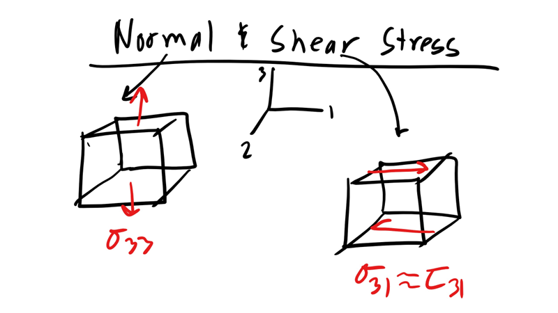
Stress, σ, is a force normalized by the area over which it acts and the force is perpendicular to the area \begin{align}\sigma = \frac{F}{A} = \frac{N}{m^2} = Pa\end{align}

where F is force and A is the original area. This is the definition of the engineering stress the true stress would be normalized by the instantaneous area. In this class we will use the engineering stress primarily in this class. Shear stress, τ, is a force normalized by the area over which it acts and the force is parallel to the area.

The shear stress is similarly defined as\begin{align}\tau = \frac{F}{A}\end{align}

Now it should be noted here that stress is a second rank tensor, σ_ij, and so is strain, ϵ_ij. For stress i denotes the normal to the plane, on which the force is acting and j is the direction of the force\begin{align}\sigma_{ij} = \frac{F_{j}}{A_{i}}\end{align}

So our full stress tensor or our most generic stress state would be \begin{align}\sigma =\begin{bmatrix}\sigma_{11} & \sigma_{12} & \sigma_{13} \\\sigma_{21} & \sigma_{22} & \sigma_{23} \\\sigma_{31} & \sigma_{32} & \sigma_{33} \\\end{bmatrix}\end{align}

Now this looks like a complex matrix with 9 independent components however they are not completely independent. If we assume that our cube volume element (representative volume element (RVE)is in equilibrium (not rotating) then we have the condition that\begin{align}\sigma_{12} = \sigma_{21}\\\sigma_{23}=\sigma_{32}\\\sigma_{31} = \sigma_{13}\end{align}

so our matrix reduces to 6 independent components for our RVE\begin{align}\sigma =\begin{bmatrix}\sigma_{11} & \sigma_{12} & \sigma_{13} \\\sigma_{12} & \sigma_{22} & \sigma_{23} \\\sigma_{13} & \sigma_{23} & \sigma_{33} \\\end{bmatrix}\end{align}

Strain:

All machines, structural members, and materials will deform to some extend when externally loaded by a force or stress. That deformation results in a displacement or strain, ϵ \begin{align}\epsilon = \frac{dL}{L}\end{align} \begin{align} \epsilon_{t} = \int_{L_1}^{L_2} \frac{dL}{L} = ln \frac{L_{2}}{L_{1}} \end{align}

where L₁ is the original length. This is the definition of true strain, ϵ_t but typically we work with a simpler form called the engineering strain, ϵ_e, \begin{align}\epsilon_{e} = \frac{L_{2}-L_{1}}{L_{1}} = \frac{\Delta L}{L_{1}} \end{align}

Typically engineers work with microstrain or parts per million. Poisson’s Ratio:

Now what happens to the dimensions perpendicular to the direction of applied force when a the material is subjected to uniaxial tension? We know from experience that a body begin pulled in tension will contract laterally. This lateral strain is described by the Poisson’s Ratio: \begin{align}\nu = -\frac{\epsilon_{L}}{\epsilon_{A}}\end{align}

where ϵ_L is the lateral strain and ϵ_A is the axial strain. Note the negative sign which signifies a decrease in length. The Poisson’s ratio is typically around 0.3 for metals, 0.5 for rubber, 0.4-0.5 for polymeric materials or biomaterials, and 0.2 for ceramics.

Stress-Strain Curve Analysis

Here we can find which material on these stress-strain curves is the most

• Stiffest

• Compliant

• Toughest

• Brittle

• Ductile

• Strongest

• Weakest

Linear Elastic Cubic Material Uniaxial Problems

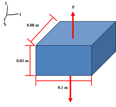
Consider the following block of aluminum and there is an applied force of 18kN in Fig.4

Calculate the following values

• Stress

• Strain

• Final Length in the 3 direction

• Final Length in the 1 direction

• Final Length in the 2 direction

Let’s do this question if now we were under compression.

Bending

There are many scenarios where an object will undergo bending and we can calculate the stress in that beam \begin{align}\sigma = -\frac{My}{I} \end{align}

where \(I = \frac{bh^3}{12}\) is the moment of inertia of a rectangular beam and \(y\) is the distance from the neutral axis of the beam.

Let us consider a classical example of a cantilever beam made of Nylon 6-6 with a length of 100cm, a width of 3cm, and a thickness of 0.1cm in Fig.5.

Let solve for the stress at the support of the wall.

Buckling

Buckling is an instability phenomenon that can occur for columns under simple uniaxial compression and the critical load for buckling is \begin{align} P_{cr} = \frac{\pi^2 E I}{l^2} \end{align}

Now in terms of what n refers to physically it is the number of half-wavelengths along a column of length l. We see several interesting but expected phenomenon in this equation the first is that the critical load for buckling is linearly dependent on the flexural modulus but also scales as l⁻2 so the longer the beam the lower the critical load which makes sense intuitively. So if we Ideally we would also want a constant I about all cross sectional axes and to have the same buckling load about all axes.