Chapter 6: Strain Gauges and Wheastone Bridges

Are The Wires Elongating or Contracting? Resistance is Futile.

The resistance of a material will change when subjected to an external strain. Consider some conductive material like a wire of copper that has some length \( l \) and diameter \( D \). If the wire is subjected to uniaxial tension along the length of the wire, as seen below, then the length will increase as diameter of the wire decreases.

This will result in a change in the resistance of the wire and specifically the resistance will increase. We can calculate this change in resistance below where \( R \) is resistance:

$$
R = \frac{\rho l}{A} = \frac{\rho l}{C D^2}
\]

where \( \rho \) is resistivity and \( C \) is a constant which will describe the cross sectional area; for a wire \( C = \frac{\pi}{4} \) for a circular cross section.

The change in resistance is then given by our old friend the chain rule:

$$
dR = \frac{dR}{d \rho} + \frac{dR}{dl} + \frac{dR}{dD} \\
dR = \frac{C D^2(l d \rho + \rho dl) - 2 C \rho lD dD}{(C D^2)^2} \\
dR = \frac{1}{C D^2} \left( l d \rho + \rho dl - 2 \rho l \frac{dD}{D} \right)
\]

If we then divide by \( R \):

$$
\frac{dR}{R} = \frac{dl}{l} - 2 \frac{dD}{D} + \frac{d \rho}{\rho} \\
\frac{\frac{dR}{R}}{\frac{dl}{l}} = 1 - 2 \frac{\frac{dD}{D}}{\frac{dl}{l}} + \frac{\frac{d \rho}{\rho}}{\frac{dl}{l}}
\]

From the equation above we can see:

$$
\epsilon_{11} = \frac{dl}{l} \\
\epsilon_{22} = \frac{dD}{D} \\
\nu = -\frac{\frac{dD}{D}}{\frac{dl}{l}}
\]

We can then define the gauge factor \( F \), which is typically determined experimentally and will typically be a constant for the problems that we will work with in this class as:

$$
F = \frac{\frac{dR}{R}}{\frac{dL}{L}} = \frac{\frac{dR}{R}}{\epsilon_{11}} = 1 + 2 \nu + \frac{\frac{d \rho}{\rho}}{\frac{dL}{L}}
\]

This equation is a bit messy as you can see but we can re-arrange this expression and get our fundamental expression for how resistance will change with strain as seen below:

$$
\epsilon_{11} = \frac{1}{F} \frac{\Delta R}{R}
\]

Here we can clearly see that the change in resistance and strain are proportional — i.e. as we strain a material in tension the resistance increases. And our strain gauge is composed of these wires as seen below and they will extend or compress depending on the applied stress:

Now at this point you may ask: why do we typically measure a voltage output from our strain gauge? Why don't we just measure the change in resistance directly? Why do I have to learn circuits, why are you so mean...

Well the answer lies once again in the precision and sensitivity of a measurement. If we are measuring microstrain we cannot use an ohmmeter to measure these values. Instead we will utilize circuits and specifically a Wheatstone Bridge Circuit and measure the corresponding change in voltage and correlate that to the strain in a material. However, before we jump directly into Wheatstone Bridge circuitry we should first begin with the building blocks of a Wheatstone Bridge which is a voltage divider circuit.

Voltage Divider Circuit

Below is a schematic of a voltage divider circuit. If we first imagine that initially there is a negligible amount of current taken from \( V_o \), our output voltage, then \( V_o \approx 0 \) and then we find that:

$$
I = \frac{V_i}{R_1 + R_2}
\]

where \( V_i \) is the input voltage. This gives us the current in our circuit, but if we find that there is current drawn from \( V_o \), then we find that:

$$
V_o = i R_2 = \frac{R_2}{R_1 + R_2} V_i
\]

This is the output for a single voltage dividing circuit.

Why did we learn about a voltage dividing circuit? You said Wheatstone bridge circuits were important for strain gauges!

Yes, I agree — but as you will see our Wheatstone Bridge Circuit will look very similar to two voltage dividing circuits.

Wheatstone Bridge Circuit

We will utilize a Wheatstone Bridge circuit to measure strain in our strain gauges, and we can see an example of Wheatstone bridges and how it looks very similar to two voltage dividing circuits.

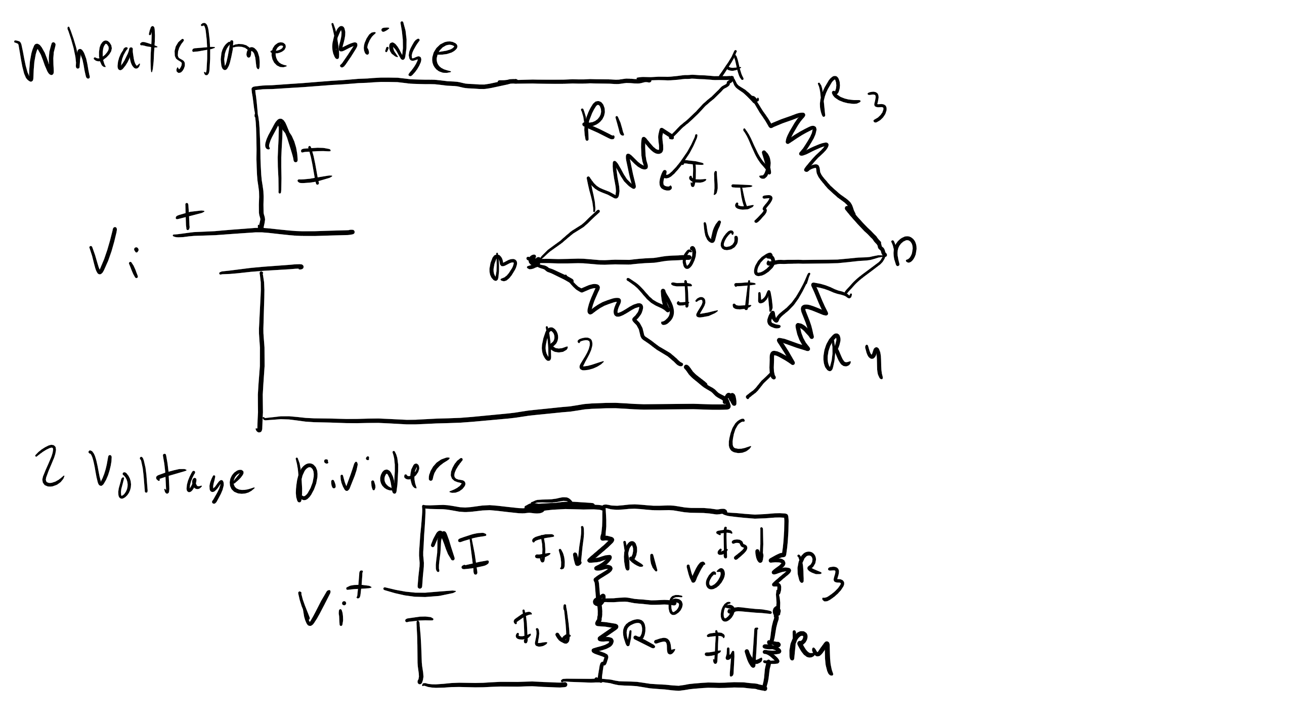
In fact, we can write out the voltage at positions 1 and 2, \( V_1 \) and \( V_2 \), and we see that the expressions are equivalent:

$$
V_1 = V_i \frac{R_2}{R_1 + R_2} \\
V_2 = V_i \frac{R_4}{R_3 + R_4}
\]

Now at balance we should find that \( V_o = 0 \), and thus \( V_1 = V_2 \). If we set these expressions equal to one another, we find:

$$
R_2 R_3 = R_1 R_4 \\
\frac{R_1}{R_2} = \frac{R_3}{R_4}
\]

If we are not at balance, we can also calculate the output voltage of the Wheatstone Bridge configuration, similar to what we did for the voltage dividing circuit:

$$
V_0 = V_1 - V_2 = V_i \left[ \frac{R_2}{R_1 + R_2} - \frac{R_4}{R_3 + R_4} \right] = V_i \left[ \frac{R_2 R_3 - R_1 R_4}{(R_1 + R_2)(R_3 + R_4)} \right]
\]

You can see in this expression that if \( R_2 R_3 = R_1 R_4 \), then we are balanced and \( V_0 = 0 \).

Now so far we have just looked at a Wheatstone Bridge circuit composed of only resistors, but we want to replace some of these resistors with strain gauges and then correlate the change in output voltage to the applied strain.

Let's start with the most general case where we replace all resistors with strain gauges, a configuration referred to as Full Bridge configuration.

Full Wheatstone Bridge in Standard Configuration

Let's look at the full Wheatstone bridge configuration as seen below:

If we replace the 4 resistors with 4 strain gauges (each must have the same resistance so that at balance the output voltage is 0), we can think of the most general case where we strain a material that has 4 strain gauges attached and consider the change in resistance and corresponding change in output voltage.

So let's begin with our expression for the output voltage for the standard Wheatstone bridge configuration:

$$
V_0 = V_i \left[ \frac{R_3}{R_1 + R_3} - \frac{R_4}{R_2 + R_4} \right]
\]

Now the change in voltage for a change in resistance for each arm will be given by the following expression:

$$
dV_0 = \frac{\partial V_0}{\partial R_1} dR_1 + \frac{\partial V_0}{\partial R_2} dR_2 + \frac{\partial V_0}{\partial R_3} dR_3 + \frac{\partial V_0}{\partial R_4} dR_4
\]

$$
\frac{dV_0}{V_i} = \frac{R_2 dR_1}{(R_1 + R_2)^2} - \frac{R_1 dR_2}{(R_1 + R_2)^2} - \frac{R_4 dR_3}{(R_3 + R_4)^2} + \frac{R_3 dR_4}{(R_3 + R_4)^2}
\]

For this course and the Wheatstone bridges we will work with, \( R_1 = R_2 = R_3 = R_4 = R \), so we can write:

$$
\frac{dV_0}{V_i} = \frac{dR_1 - dR_2 - dR_3 + dR_4}{4R}
\]

And remembering back to our fundamental equation:

$$
\epsilon_n = \frac{1}{F} \frac{\Delta R}{R}
\]

Substituting in, we can get our final, critical, and fundamental expression for relating output voltage and strain using Wheatstone bridges as seen below:

<img src="standard2.png" alt="Standard Wheatstone Bridge Configuration Fundamental Equation." />

$$
\frac{dV_0}{V_i} = \frac{F}{4} \left[ \epsilon_1 - \epsilon_2 - \epsilon_3 + \epsilon_4 \right]
\]

We can now use this expression to describe the relationship between the output voltage, strain, and stress for a myriad of different strain gauge configurations. Let's consider several examples to illustrate how we will utilize this expression.

Strain Gauge Configuration

Uniaxial Tension Quarter Bridge Configuration

If we consider a Quarter Bridge Configuration (only 1 strain gauge in our bridge) as seen below:

So we have a strain gauge in the 1 arm of our Wheatstone bridge and it is aligned with \( \sigma_{11} \). Now remember if the wires extend/elongate that correlates to a positive strain and because we only have one strain gauge the resistors in the 2, 3, and 4 arms are not being stretched so the strain there is 0. Furthermore, we know that the strain measured in the 1 arm will just be \( \epsilon_1 = \epsilon_{11} \). Aren't you glad we covered mechanics first?

Let's do another example where now we have an additional stress, \( \sigma_{22} \).

Well everything else holds in this example but our expression for \( \epsilon_{11} \) changes and now it is:

$$
\epsilon_{11} = \frac{\sigma_{11}}{E} - \frac{\nu \sigma_{22}}{E}
\]

Notice the additional negative component in this strain because as the material is stretched in the 22 direction, the wires will compress and the length will decrease — thus the negative sign.

Let's look at the same stress state but add another strain gauge to make a Half-Bridge configuration as seen below:

Here now we have a strain gauge aligned with the 22 direction so it will sense \( \epsilon_{22} \), so:

$$
\epsilon_2 = \epsilon_{22}
\]

Alright, you are now masters of tension, compression, and normal stress — but what about bending?

Let's take a look at the scenario below of a cantilever beam bending:

Here we again only have one strain gauge, but now it will be exposed to pure bending strain, and this strain will be positive if the strain gauge is on top of the beam (denoted by a solid outline of the strain gauge) because the wires will elongate.

However, in the figure below you can see that if we have a strain gauge placed on the bottom of the beam then the wires will compress and that will correlate to a negative bending strain. So be ready for some examples with normal and bending strain combined... I know I know so mean.

Linear Thermal Expansion Contribution to Strain

Thus far we have neglected one contribution to strain and that is the contribution of thermal strain. Most materials (see exceptions like PbTiO₃ and other materials with a negative thermal expansion coefficient) will expand as temperature increases, and this behavior is reflected in a material's linear thermal expansion coefficient described below:

$$
\alpha_L = \frac{1}{L}\frac{dL}{dT}
\]

We can re-write this expression to obtain the thermal strain \( \epsilon_{\text{thermal}} \):

$$
\epsilon_{\text{thermal}} = \frac{\Delta L}{L} = \alpha_L \Delta T
\]

This thermal strain will cause the wires in the strain gauge to expand, and thus this contribution will typically always be a positive contribution to strain (unless \( \alpha_L \) is negative). You can also configure your strain gauges in such a manner to eliminate the thermal strain contribution if you do not want to measure that contribution.

Calibration of Strain Gauges

Way way back in lecture one we mentioned that when designing experiments or making an experimental apparatus, calibration was a critical step. The same calibration must be performed for strain gauges as well. However, this is a difficult proposition.

As you might imagine, calibration will involve placing a strain gauge on a material and applying a fixed strain and measuring the resulting output voltage. This is a valid way to calibrate — but as uncertainty experts think about all the potential uncertainties that can occur in this process:

- Uncertainty in the applied strain
- Defects in the material
- Variation in geometry and dimensions
- Error introduced by the mounting process itself

Instead, we will utilize an ingenious calibration technique which involves the precise application of a known change in resistance and measuring the system's response.

To do this, we add a switch \( S \) and a shunt resistor \( R_S \) to the 1-arm of our Wheatstone Bridge:

When the switch is open, the resistance in arm 1 is just \( R_1 \). When the switch is closed, the resistance changes to:

$$
\frac{R_1 R_S}{R_1 + R_S}
\]

So the change in resistance after closing the switch is:

$$
\Delta R = \frac{R_1 R_S}{R_1 + R_S} - R_1 = -\frac{R_1^2}{R_1 + R_S}
\]

And remembering:

$$
\epsilon = \frac{1}{F}\frac{\Delta R}{R}
\]

We find the corresponding strain from the change in resistance is:

$$
\epsilon = \left| -\frac{1}{F} \left( \frac{R_1}{R_1 + R_S} \right) \right|
\]

Full Wheatstone Cantilever Beam Bending

Consider an Al-6061 cantilever beam with full Wheatstone Bridge Configuration as seen below. The gauge factor is 2 and the excitation voltage is 5 V. The beam thickness is 0.1 m and the length is 10 m. The initial resistances in each arm of the Wheatstone Bridge are 120 Ω. What is the change in voltage after this load is applied?

Write Out the Strain

Let's look at the following material under a combination of uniaxial tension and bending:

Write out the strain in each strain gauge.

Determine the configuration that eliminates bending.

Determine the configuration which eliminates axial strain components.

I Can't Stop Asking Thin Walled Pressure Vessel Problems

Take a look at the arrangement of strain gauges on the cylindrical vessel seen below:

Consider an aluminum pressure vessel with full bridge configuration as seen below. The thickness is 0.1 m. The initial resistances of the strain gauges are 200 Ω. The gauge factor is 4. Initially a shunt is placed across gauge 1 and the output reads 20 units (your oscilloscope is so old you cannot read the units). After the cylinder is pressurized you read an output of 50.

Calculate the hoop and longitudinal stress.

Strain Rosettes: Rectangular and Delta

For the examples that we have done so far, our strain gauges have been aligned with our coordinate system or along principal directions. But if we want to measure a complex stress state — where a plane stress condition is completely unknown, like near a weld, defect, microcrack, etc. — we will need to utilize 3 strain gauges and then use Mohr's circle for our strain tensor to determine the normal and shear strains (as our strain gauges cannot directly measure shear strains — they only give us normal strains).

This configuration of 3 strain gauges is called a strain rosette. There are multiple types of rosettes (T-Delta), but in this course we will focus on rectangular and delta or equiangular rosettes as seen below:

You can see that for the rectangular rosette the a and b arms are offset by \( 45^\circ \) as are b and c, and the a and c arms are offset by \( 90^\circ \). For the delta rosette the a and b arms are offset by \( 60^\circ \), b and c are offset by \( 60^\circ \), and a and c arms are offset by \( 120^\circ \).

Now let's imagine that we place a rectangular rosette on a material near a weld, defect, stress concentrator, etc., i.e. near any complex stress state we may not know. If we place the rectangular rosette there and apply the load for that particular application, we will obtain strain readings from each arm of the rosette.

If we find that \( \epsilon_a = 72 \), \( \epsilon_b = 120 \), \( \epsilon_c = 248 \) in microstrain, we can then calculate the principal strains, stresses, rotation to get to the principal strain state, the center of our Mohr's circle, and the radius of our Mohr's circle.

Sounds like a lot of work right? But you are masters of Mohr's circle and rotation so this will be very similar — but with one key distinction: we need to perform our Mohr's circle in strain as seen below.

Now we just mentioned that our strain gauges cannot measure shear strains directly, so thus any measurement from each arm can be considered a normal strain.

Now for our stress state in Mohr's circle, we had coordinates and drew our circle that way because we knew the normal and shear stresses. But here we only know the x-values — i.e., our normal strains.

But we know that our Mohr's circle must intersect these vertical normal strain lines at six points as seen in the figure.

We also know that we have three unknowns in our Mohr's circle:
- Center \( c \)
- Radius \( R \)
- \( 2\theta \)

But we know \( \epsilon_A \), \( \epsilon_B \), and \( \epsilon_C \), so we can use our circle geometry to solve for these unknowns.

From the figure we see the relationship that relates \( \epsilon_A \) to \( c \), \( R \), and \( 2\theta \):

$$
\epsilon_A = 72 \times 10^{-6} = c + R \cos(2\theta)
\]

We can also obtain a relationship for \( \epsilon_B \) and \( \epsilon_C \), knowing that they are offset by a fixed angle from arm A. We know that for B in real space the angle is \( 45^\circ \), but in Mohr's circle that translates to \( 90^\circ \), so we add this to our expression:

$$
\epsilon_B = 120 \times 10^{-6} = c + R \cos(2\theta + 90^\circ)
\]

Similarly for arm C:

$$
\epsilon_C = 248 \times 10^{-6} = c + R \cos(2\theta + 180^\circ)
\]

With these three equations we can solve for our unknowns and find that:

$$
c = 1.6 \times 10^{-4} \\
R = 9.6 \times 10^{-5} \\
\epsilon_1 = 2.6 \times 10^{-4} \\
\epsilon_2 = 6.33 \times 10^{-5} \\
\theta = 12.22^\circ \\
\sigma_1 = 6.27 \times 10^7 \, \text{Pa} \\
\sigma_2 = 3.19 \times 10^7 \, \text{Pa}
\]

We can obtain our principal stresses from our stress tensor and strain tensor relationships:

$$
\epsilon_1 = \frac{1}{E}(\sigma_1 - \nu \sigma_2) \\
\epsilon_2 = \frac{1}{E}(\sigma_2 - \nu \sigma_1)
\]

You can use this framework to calculate many different stress and strain states. For the delta rosette, we would perform a similar procedure but the angles would be different — i.e. \( 60^\circ \) instead of \( 45^\circ \). Also, you can imagine I might/will give you a different rosette on a Pset or an Exam and you might have to do even more rotations...