Chapter 7: Introduction to Feedback Control, Laplace Transforms, and Transfer Functions

Introduction to Feedback Control

Control systems are a fundamental component of modern engineering design. Applications range across disciplines, including aircraft stabilization, robotic surgery, precision manufacturing, and temperature regulation in chemical reactors. In all cases, the objective remains the same: to automatically manipulate a system’s behavior so that it conforms to a prescribed performance or reference trajectory.

A control system achieves this by continuously measuring the system’s output, comparing it to a desired input, and adjusting internal inputs or forces in real time to minimize the error. This process relies on feedback.

Mathematical Modeling

Designing any control system begins with developing an appropriate mathematical model of the physical system. This model typically takes the form of an ordinary differential equation (ODE), which is derived based on the system’s mechanical, electrical, thermal, or fluid characteristics. The model encapsulates effects such as:

- Inertial resistance to motion
- Elastic restoring forces
- Energy dissipation via damping
- External forcing or actuation

The resulting system dynamics are then expressed in either time-domain or Laplace-domain representations, allowing for analysis and controller synthesis using established control theory frameworks.

Prerequisite Knowledge: Dynamics

Because the systems under consideration are inherently dynamic, changing in response to inputs over time, a strong foundation in engineering dynamics is required. Students must be comfortable deriving and manipulating ODEs that describe system behavior. For example, the standard second-order linear differential equation that describes a forced mass-spring-damper system is a classic system that we will analyze in depth throughout this class:

$$
m\ddot{x}+c\dot{x}+kx=f(t)
\]

where \( m \) is the mass, \( c \) is the damping coefficient, \( k \) is the spring constant, and \( f(t) \) is the external forcing function.

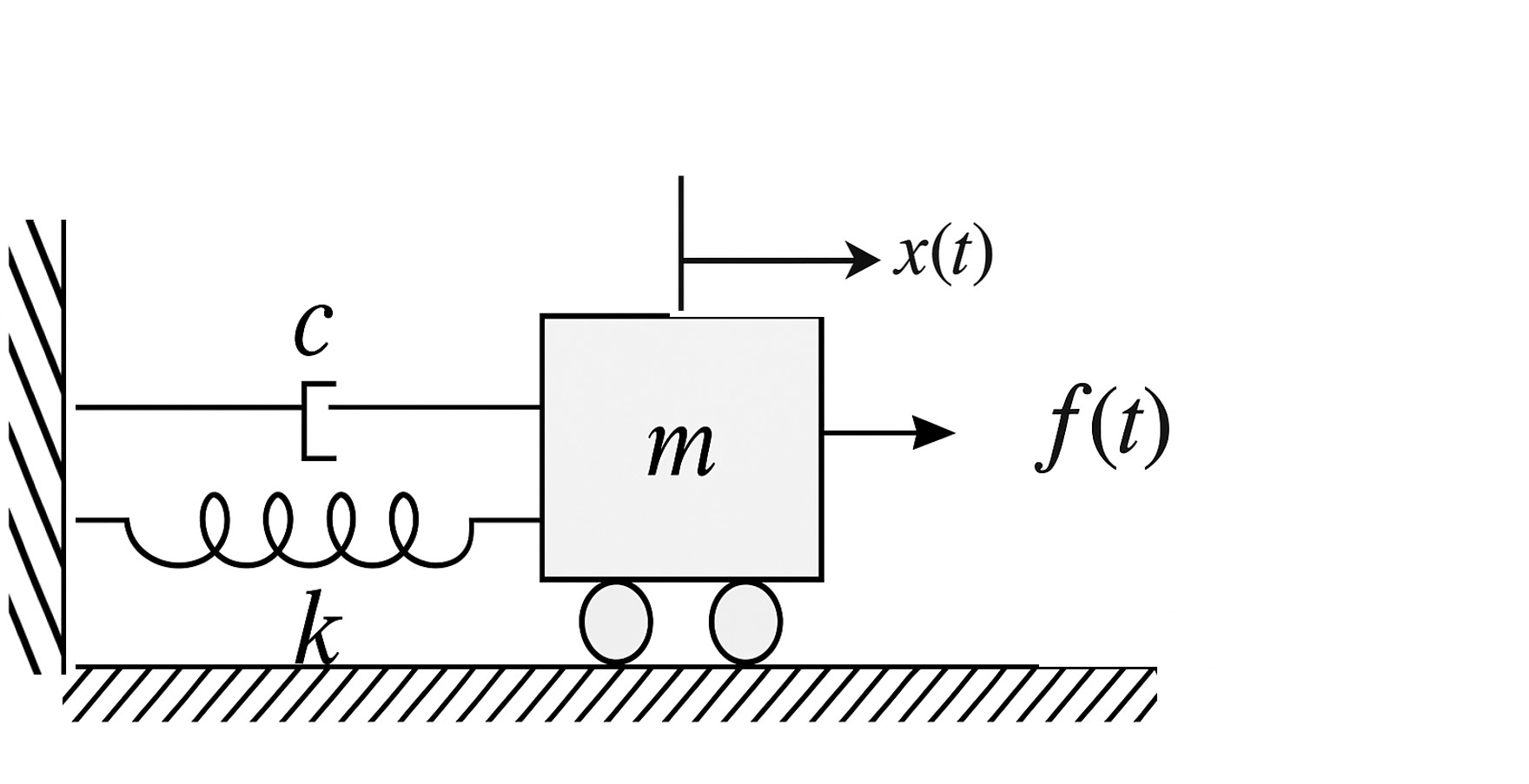
This system will appear frequently in mechanical system modeling and must be understood in terms of both its physical meaning and mathematical properties.

Two-Degree-of-Freedom Vertical Suspension Model

This simplified vertical suspension model captures the dynamic interaction between two vertically aligned masses: a lower mass (e.g., wheel and axle) and an upper mass (e.g., car chassis). The system is designed to model how a suspension system responds to vertical disturbances such as road irregularities.

The model consists of:

- \( m_1 \): the lower mass (unsprung mass), representing the wheel and axle
- \( m_2 \): the upper mass (sprung mass), representing the chassis and vehicle body

The following elements connect the components:

- A spring of stiffness \( k_1 \), connecting \( m_1 \) to the inertial ground at position \( x_0 \)
- A spring of stiffness \( k_2 \), connecting \( m_1 \) to \( m_2 \)
- A damper with damping coefficient \( c \), also between \( m_1 \) and \( m_2 \)

Define the vertical displacements as absolute positions measured from the inertial ground:

- \( x_1(t) \): absolute vertical displacement of \( m_1 \)
- \( x_2(t) \): absolute vertical displacement of \( m_2 \)
- \( x_0 \): fixed vertical position of the inertial ground (typically set to zero)

Rotational Dynamics

Rotational systems obey Newton’s second law in angular form:

$$
\sum \tau = J \alpha = J \ddot{\theta}(t)
\]

where:

- \( \tau \) is net torque applied to the system
- \( J \) is the moment of inertia about the axis of rotation
- \( \theta(t) \) is the angular position

Analogous to mass-spring-damper translational systems, we can add:

$$
J \ddot{\theta} + b \dot{\theta} + k \theta = \tau(t)
\]

Here, \( b \) is torsional damping and \( k \) is angular stiffness (e.g., from torsional springs).

This is structurally identical to the mass-spring-damper system — all the second-order analysis tools (natural frequency, damping ratio, etc.) apply directly.

Pendulum and Inverted Pendulum

A pendulum is a prototypical nonlinear system. Consider a simple pendulum of mass \( m \), length \( L \), with angular displacement \( \theta(t) \) from vertical.

The torque due to gravity is:

$$
\tau = -mgL \sin(\theta)
\]

Using \( \sum \tau = J \ddot{\theta} \) and \( J = mL^2 \), we get:

$$
mL^2 \ddot{\theta} + mgL \sin(\theta) = 0
\Rightarrow
\ddot{\theta} + \frac{g}{L} \sin(\theta) = 0
\]

This is a nonlinear second-order ODE.

Inverted Pendulum:

The pivot is below the mass — the torque due to gravity is destabilizing.

$$
\ddot{\theta} - \frac{g}{L} \theta = 0
\Rightarrow
\theta(t) = \theta_0 e^{\sqrt{g/L} \, t}
\]

This exhibits exponential divergence — instability. Such a system cannot balance itself without feedback. This is the same principle as balancing a stick on your palm (see earlier lecture section).

Inverted pendulums are central in many modern control labs: Segways, rockets, cart-pole systems, and humanoid robotics.

Gears and Gear Trains

Gears convert rotational motion and torque between shafts. For gears with radii \( r_1, r_2 \) and number of teeth \( N_1, N_2 \), the gear ratio is:

$$
n = \frac{N_2}{N_1} = \frac{r_2}{r_1} = \frac{\omega_1}{\omega_2}
\quad \text{and} \quad
\tau_2 = n \tau_1
\]

Key principles:

- Angular displacement and velocity are inversely related to gear ratio
- Torque is multiplied by gear ratio

When modeling systems with gears, it’s useful to reflect all inertias and torques to a common shaft. For instance, to reflect \( J_2 \) to shaft 1:

$$
J_{\text{eq}} = J_1 + n^2 J_2
\]

This simplifies the system to a single equivalent inertia. Similar transformations apply to damping and stiffness.

First-Order Thermal System (Lumped Heat Transfer)

A common thermal model is a lumped body exchanging heat with the ambient through a thermal resistance \( R \), having thermal capacitance \( C \). Let \( T(t) \) be the body temperature, \( T_a(t) \) the ambient.

$$
C \frac{dT}{dt} = -\frac{1}{R}(T - T_a)
\]

This is a first-order system with time constant \( \tau = RC \). The system exponentially approaches ambient temperature. This same structure models RC electrical circuits, fluid tanks, and population decay.

Unity Feedback Configuration

This course begins with the unity feedback configuration, a canonical architecture in control theory. While more complex architectures exist, the unity feedback structure is sufficiently general to illustrate core principles and to control a wide range of systems.

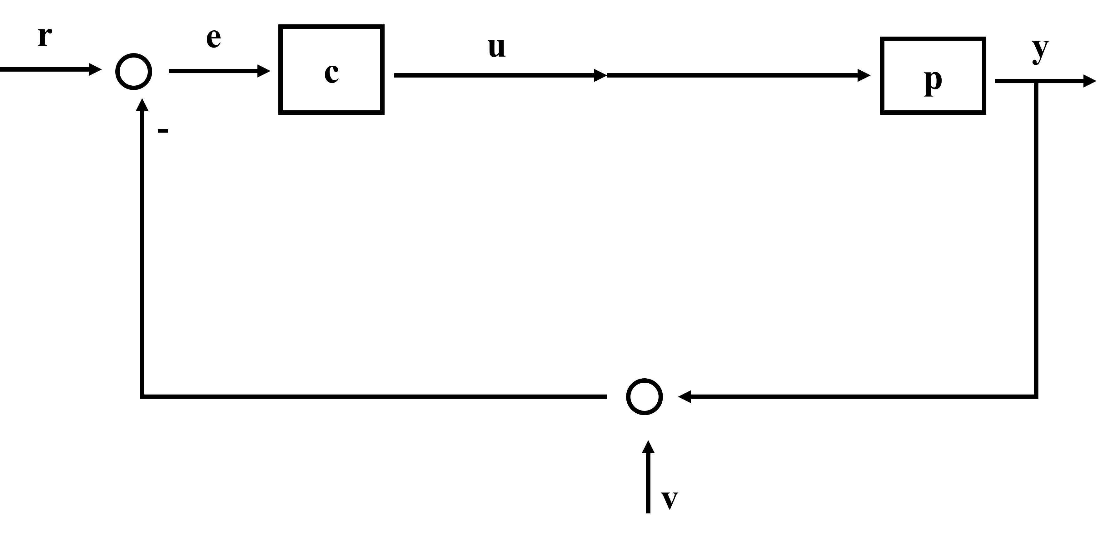
In a unity feedback system, the output is subtracted from the reference input to form the error signal. This error is then fed to a controller, which applies a control input to the plant. The plant output is measured and looped back to be compared with the input. This closed-loop configuration is illustrated here:

There are several critical components to the block diagram and inputs and outputs, much more on that later. One major component or block in this diagram is the plant, \( p \), which is our dynamic system that we are trying to control. This could be a robot, temperature control, pendulum, etc. \( y \) is the measured output of our system and it is the variable that we are trying to control and it will be measured with a sensor. \( r \) is the reference or the signal that we want, i.e. the desired output. \( e \) is the error and is simply the difference between \( r \) and \( y \):

$$
e = r - y
\]

\( c \) is the controller and we will spend a lot of the class to develop this. The output from the controller is \( u \), the control command, and is the input to the plant via some type of actuator which can be some type of motor or other actuator.

The goals of feedback controls are:

- Stability
- Tracking: system output must track the reference signal as close as possible
- Disturbance rejection: system output must be as insensitive as possible to disturbance inputs
- Robustness

Now this may seem very abstract so let's put this in the context of an example that we will come back to over and over and over again in this class so learn to love this example — and that is cruise control in a car.

For this application, we set a particular speed, say 65 mph — that will be our reference, \( r \). The actual speed of the car would be \( y \) and is measured via a sensor, perhaps some type of conversion of tire rotation to translational displacement. The error \( e \) is just the difference between these two signals. The plant \( p \) in this example would be the vehicle. The cruise control will take the signal from the error and then send a control command \( u \) to the actuator, which will be the accelerator or something of the like.

Let's think about another example like a Segway, which is similar to an example and lab we will conduct in this course which is an inverted pendulum where we actually use unstable dynamics to drive around. For a Segway we want to remain balanced, so our measured output \( y \) will be the angle between the Segway and the vertical line perpendicular to the surface. We want the reference \( r \), or that angle, to be \( 0^\circ \) and the control command will control the motor torque to the Segway wheel.

You can extend this to HVAC systems where the plant is the house, the \( y \) is the measured temperature, \( r \) is the desired temperature, and the control command will be sent to the AC damper or a valve control.

This feedback loop introduces several critical properties:

- Improved disturbance rejection
- Reduced steady-state error
- Enhanced tracking performance
- Robustness to model uncertainties

Block Diagram Analysis

Throughout this course, feedback control systems will be analyzed using block diagrams. These diagrams abstract the mathematical operations of each subsystem, allowing for algebraic manipulation of entire control loops using transfer functions. This simplifies stability analysis, error dynamics, and sensitivity functions, particularly in the frequency domain.

Feedback control is essential for the design and stabilization of dynamic systems, particularly those that are unstable in their natural configuration. To understand the role of feedback, consider the consequences of removing the feedback path in a control loop. If we eliminate the sensor and the associated feedback signal, the system becomes an open-loop configuration. This configuration lacks the capability to automatically correct deviations between the desired and actual outputs.

To illustrate this, consider the classic example of balancing a stick vertically on your palm. In the context of a unity feedback control system (so named because the feedback signal is directly subtracted from the reference), we can identify the following components:

- Plant: the stick, which is inherently unstable when balanced upright
- Output \( y(t) \): the angular deviation of the stick from the vertical axis
- Reference \( r(t) \): the desired angle, ideally \( r(t) = 0^\circ \)
- Sensor: your eyes, providing visual feedback
- Controller \( C \): your brain, processing the error
- Actuator: your arm or hand muscles
- Control input \( u(t) \): the motion applied to keep the stick upright

In this feedback loop, you continuously observe the angle \( y(t) \), compare it to the reference \( r(t) \), and apply corrective motion \( u(t) \) to minimize the error.

Now consider removing the sensor — closing your eyes. This breaks the feedback loop. Without sensory input, the controller has no error information and cannot generate a meaningful corrective action. As a result, the plant becomes unstable and the stick falls. This demonstrates a key point: without feedback, inherently unstable systems cannot be stabilized.

Open-Loop Control Systems

In an open-loop system, there is no feedback: the controller sends an input to the actuator, which influences the plant, and the output is observed without adjustment. The error signal \( e(t) = r(t) - y(t) \) is not computed or used.

Such systems are viable only under specific conditions, primarily when the plant dynamics are well understood, repeatable, and stable. Since no corrections are made based on the output, open-loop control cannot adapt to disturbances or uncertainty.

A common example is a toaster:

- Plant: the toaster, with thermal dynamics governed by heat transfer
- Controller: the knob, regulating time or power level
- Actuator: the heating element
- Output \( y(t) \): the toast produced
- Reference \( r(t) \): desired doneness, e.g., golden brown

There is no feedback, no sensor measures toast color or crispness. If the bread changes (e.g., frozen vs. fresh, thin vs. thick), the system cannot adapt. Manual adjustments are required, and the output becomes inconsistent. For this reason, open-loop control is rarely suitable for complex or sensitive systems.

Closed-Loop Control Systems

In contrast, closed-loop (feedback) control systems incorporate real-time measurement and comparison between the desired output \( r(t) \) and the actual output \( y(t) \). The difference, the error signal \( e(t) = r(t) - y(t) \), is used by the controller to determine the appropriate control input.

This architecture enables:

- Stabilization of unstable systems
- Performance improvement in already stable systems
- Robustness against disturbances and modeling uncertainty
- Tuning of speed, overshoot, and steady-state error

In feedback systems, controller design focuses on shaping system behavior to meet specific performance specifications, often involving trade-offs between speed of response, stability margins, and sensitivity to disturbances.

Understanding the dynamics of the plant is essential in control system design. The plant is the component of a feedback system that we are trying to control, typically a physical, dynamic system. To analyze such systems effectively, a solid foundation in dynamics is required.

A dynamic system is characterized by a time-dependent input-output relationship, where the output at the current time depends not only on the current input but also on past inputs and system states. In other words, dynamic systems have memory.

Consider the example of riding a bicycle. The input \( u(t) \) is the torque applied by pedaling, and the output \( y(t) \) is the bicycle’s velocity. Even if pedaling ceases, the bicycle may continue to coast — this demonstrates that the current velocity depends on prior input. This is a classic example of a first-order dynamic system.

Car Velocity Plant Function

Let us now consider a more formal example involving a car. The control input \( u(t) \) is the throttle angle, and the system output \( y(t) \) is the vehicle’s velocity. Clearly, the input and output are not linearly or instantaneously related — this is a dynamic system.

To study this system properly, we need to characterize how the input affects the output over time. That is the role of dynamic system modeling. Specifically, we want to develop a mathematical model that captures the behavior of the system using differential equations.

For this course, we will primarily focus on mechanical dynamic systems, and thus we will rely heavily on Newton's Second Law and free-body diagrams (FBDs) as our modeling tools. While control systems can span other physical domains (e.g., electrical systems using Kirchhoff’s laws), our examples will primarily involve translational mechanical systems.

Let us model the car using a simplified, one-dimensional representation. The assumptions are:

- The vehicle has mass \( m \)
- The input is the forward thrust force from the engine \( u(t) \)
- The resisting force is aerodynamic drag, modeled as \( F_d = b v(t) \), where \( b \) is a damping (drag) coefficient
- The output is velocity \( v(t) \)

We apply Newton’s Second Law in the direction of motion:

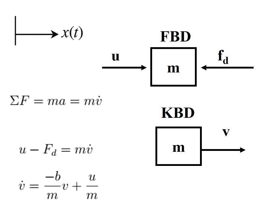
$$
\sum F = ma = m\dot{v}(t)
\]

$$
u(t) - F_d = m\dot{v}(t)
\]

$$
u(t) - b v(t) = m\dot{v}(t)
\]

Rearranging, we obtain the first-order linear ordinary differential equation (ODE):

$$
\dot{v}(t) = -\frac{b}{m}v(t) + \frac{1}{m}u(t)
\]

This ODE captures the complete input-output dynamics of the system. It holds for arbitrary inputs, including impulse, step, or sinusoidal signals.

Let us examine the case of a constant step input \( u(t) = 1 \):

$$
u(t) = 1 \quad \text{(unit step input)}
\]

Solving the ODE with zero initial conditions yields:

$$
v(t) = \frac{1}{b} \left(1 - \exp\left(-\frac{b t}{m}\right)\right)
\]

This solution exhibits first-order exponential behavior, consistent with physical intuition: the velocity increases over time and asymptotically approaches a steady-state value determined by the balance between thrust and drag.

From Time Domain to Laplace (s) Domain

While time-domain modeling is fundamental, it is often advantageous to work in the Laplace domain. In this domain, differential equations become algebraic equations, and system behavior can be represented using transfer functions.

- The physical system exists in the real world.
- The time-domain model is a differential equation derived from physics.
- The Laplace-domain model is an algebraic representation via the transfer function.

These three boxes describe the same system in different but equivalent forms. The Laplace transform is the tool that lets us move between the time and frequency (s) domains. Mastery of both domains is essential for modern control analysis and design.

Laplace Transforms and Transfer Functions

To control a system, we must first understand and model its dynamic behavior. The plant refers to the system we aim to control. Through the process of modeling—usually based on Newton’s Second Law—we obtain a set of ordinary differential equations (ODEs) that describe the plant’s dynamics.

However, solving ODEs in the time domain can be analytically difficult and computationally expensive. To simplify the analysis, we often convert the system to the Laplace domain (s-domain) using the Laplace transform. This conversion allows us to represent dynamic relationships algebraically rather than differentially.

The Laplace transform of a time-domain function \( f(t) \) is defined as:

$$
F(s) = \mathcal{L}\{f(t)\} = \int_0^{\infty} f(t) e^{-st} \, dt
\]

This operation transforms a time-domain function into an algebraic function of the complex variable \( s \), greatly simplifying the manipulation of dynamic system models.

Transfer Function Definition

Let \( u(t) \) be the input to a dynamic system and \( y(t) \) be the corresponding output. The transfer function \( H(s) \) is defined as:

$$
H(s) = \frac{\mathcal{L}\{y(t)\}}{\mathcal{L}\{u(t)\}} = \frac{Y(s)}{U(s)}
\]

This definition assumes that all initial conditions are zero.

Procedure Overview: The Four Core Applications of the Laplace Transform

1. Derive the ODE using physical laws (e.g., Newton’s Second Law)
2. Take the Laplace transform of the ODE (with zero initial conditions)
3. Solve for the transfer function \( H(s) = \frac{Y(s)}{U(s)} \)
4. Perform inverse Laplace transforms as needed to return to the time domain

Worked Example: First-Order Car Model

Consider the simplified car model:

$$
m\dot{v}(t) + b v(t) = u(t)
\]

Taking the Laplace transform of both sides (assuming zero initial velocity):

$$
m s V(s) + b V(s) = U(s)
\]

Factor \( V(s) \):

$$
V(s)(ms + b) = U(s) \quad \Rightarrow \quad
H(s) = \frac{V(s)}{U(s)} = \frac{1}{ms + b}
\]

This is the transfer function of the system, describing how the velocity responds to the input throttle signal.

Solving an ODE via Laplace Transform

Consider the ODE:

$$
\dot{v}(t) + 2v(t) = u(t), \quad v(0) = 0
\]

Take Laplace transform:

$$
sV(s) + 2V(s) = U(s)
\quad \Rightarrow \quad V(s)(s+2) = U(s)
\quad \Rightarrow \quad V(s) = \frac{U(s)}{s+2}
\]

Let \( u(t) = 1 \) (unit step), so \( U(s) = \frac{1}{s} \). Then:

$$
V(s) = \frac{1}{s(s+2)}
\]

Use partial fraction decomposition:

$$
\frac{1}{s(s+2)} = \frac{A}{s} + \frac{B}{s+2}
\Rightarrow A = \frac{1}{2}, \quad B = -\frac{1}{2}
\]

$$
V(s) = \frac{1}{2} \left( \frac{1}{s} - \frac{1}{s+2} \right)
\]

Take inverse Laplace transform:

$$
v(t) = \frac{1}{2}(1 - e^{-2t})
\]

This matches the solution we obtained earlier by directly solving the differential equation.

Frequency Response Interpretation from Transfer Functions

Control engineers often want to understand how a system responds to sinusoidal inputs of varying frequencies. This is essential for designing controllers that reject disturbances or track desired inputs. The frequency response characterizes how each frequency component of an input signal is altered (amplified/attenuated and phase-shifted) by the system.

To analyze this, we evaluate the transfer function \( H(s) \) at \( s = j\omega \), where \( \omega \) is a real-valued angular frequency in radians per second. This gives the frequency response of the system:

$$
H(j\omega) = |H(j\omega)| e^{j\phi(\omega)}
\]

This complex number encodes two key pieces of information:

- Magnitude response \( |H(j\omega)| \): the amplitude gain of the output relative to the input
- Phase response \( \phi(\omega) \): the phase lag or lead introduced by the system

First-Order Low-Pass System

Let:

$$
H(s) = \frac{1}{\tau s + 1} \Rightarrow H(j\omega) = \frac{1}{1 + j\omega \tau}
\]

Magnitude:

$$
|H(j\omega)| = \frac{1}{\sqrt{1 + (\omega \tau)^2}}
\]

Phase:

$$
\phi(\omega) = -\tan^{-1}(\omega \tau)
\]

Low-frequency behavior: \( \omega \ll \frac{1}{\tau} \)

$$
|H(j\omega)| \approx 1, \quad \phi(\omega) \approx 0^\circ
\]

High-frequency behavior: \( \omega \gg \frac{1}{\tau} \)

$$
|H(j\omega)| \rightarrow 0, \quad \phi(\omega) \rightarrow -90^\circ
\]

Underdamped Second-Order System

Consider:

$$
H(s) = \frac{\omega_n^2}{s^2 + 2\zeta \omega_n s + \omega_n^2}
\]

Evaluating at \( s = j\omega \):

$$
H(j\omega) = \frac{\omega_n^2}{(\omega_n^2 - \omega^2) + j(2\zeta \omega_n \omega)}
\]

Magnitude:

$$
|H(j\omega)| = \frac{\omega_n^2}{\sqrt{(\omega_n^2 - \omega^2)^2 + (2\zeta \omega_n \omega)^2}}
\]

Phase:

$$
\phi(\omega) = -\tan^{-1}\left(\frac{2\zeta \omega_n \omega}{\omega_n^2 - \omega^2}\right)
\]

Key behaviors:

- Peak occurs near \( \omega = \omega_n \) if \( \zeta < \frac{1}{\sqrt{2}} \)
- Phase shifts from 0° to -180°

Why Frequency Response Matters

- Filter Design: shaping gain to attenuate noise/disturbances
- Resonance Control: identifying and avoiding frequencies that cause large oscillations
- Stability Margins: gain and phase margins directly measurable on Bode plots
- Loop Shaping: designing feedback controllers (e.g., lead/lag compensators)

Block Diagram Algebra and Transfer Function Derivations

In a typical feedback control system, we define:

- \( R(s) \): Reference input
- \( C(s) \): Controller transfer function
- \( P(s) \): Plant transfer function
- \( Y(s) \): Output
- \( E(s) = R(s) - Y(s) \): Error signal
- \( U(s) = C(s) E(s) \): Control effort
- \( D(s) \): Disturbance input (additive before plant)
- \( N(s) \): Measurement noise (additive after plant)

We now derive transfer functions for different scenarios using block diagram algebra.

1. Open-Loop Transfer Function (No Feedback)

Assume no feedback loop. The signal path is simply:

Then:

$$
U(s) = C(s) R(s), \quad Y(s) = P(s) U(s) = P(s) C(s) R(s)
\]

Open-loop transfer function:

$$
\frac{Y(s)}{R(s)} = C(s) P(s)
\]

This is often denoted:

$$
L(s) = C(s) P(s)
\]

2. Closed-Loop Transfer Function (Unity Feedback)

Now assume unity feedback and no disturbance or noise:

$$
E(s) = R(s) - Y(s), \quad U(s) = C(s) E(s) = C(s)[R(s) - Y(s)], \quad Y(s) = P(s) U(s)
\]

Substitute:

$$
Y(s) = P(s) C(s) [R(s) - Y(s)] \Rightarrow Y(s) + P(s) C(s) Y(s) = P(s) C(s) R(s)
\]

Factor:

$$
Y(s) [1 + C(s) P(s)] = C(s) P(s) R(s)
\Rightarrow
\frac{Y(s)}{R(s)} = \frac{C(s) P(s)}{1 + C(s) P(s)}
\]

3. Output Transfer Function with Disturbance \( W(s) \)

Disturbance \( W(s) \) is added before the plant:

$$
U(s) = C(s) [R(s) - Y(s)]
\Rightarrow Y(s) = P(s) U(s) + P(s) W(s)
\]

Substitute:

$$
Y(s) = P(s) C(s) [R(s) - Y(s)] + P(s) W(s)
\Rightarrow Y(s)[1 + C(s) P(s)] = C(s) P(s) R(s) + P(s) W(s)
\]

Final expression:

$$
Y(s) = \frac{C(s) P(s)}{1 + C(s) P(s)} R(s) +
\frac{P(s)}{1 + C(s) P(s)} W(s)
\]

4. Output Transfer Function with Measurement Noise \( V(s) \)

Now let \( V(s) \) be added to the measured output before it feeds back to the controller:

$$
E(s) = R(s) - [Y(s) + V(s)], \quad U(s) = C(s) E(s)
\]

Substitute:

$$
U(s) = C(s)[R(s) - Y(s) - V(s)], \quad Y(s) = P(s) U(s)
\]

$$
Y(s) = P(s) C(s)[R(s) - Y(s) - V(s)]
\Rightarrow Y(s)[1 + C(s) P(s)] = C(s) P(s) R(s) - C(s) P(s) V(s)
\]

Final expression:

$$
Y(s) = \frac{C(s) P(s)}{1 + C(s) P(s)} R(s) -
\frac{C(s) P(s)}{1 + C(s) P(s)} V(s)
\]

5. General Case with \( R(s) \), \( W(s) \), and \( V(s) \)

Now we consider the most complete block diagram, where the system is influenced by:

- \( R(s) \): Reference signal
- \( W(s) \): Disturbance (e.g., wind, vibration)
- \( V(s) \): Measurement noise

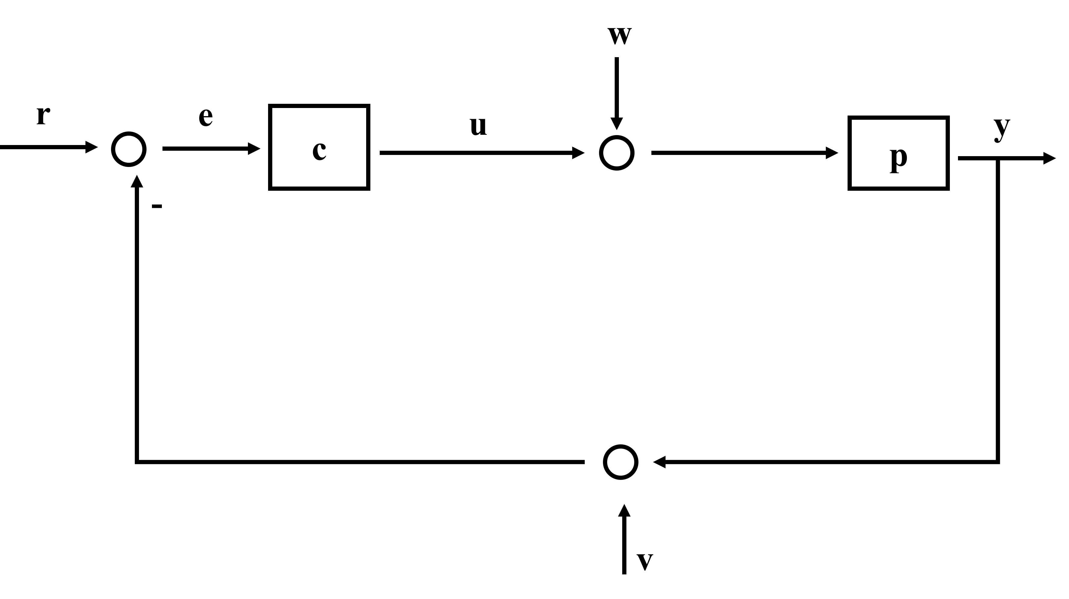
We combine everything from the previous derivations:

$$
Y(s) = \frac{C(s) P(s)}{1 + C(s) P(s)} R(s) +
\frac{P(s)}{1 + C(s) P(s)} W(s) -
\frac{C(s) P(s)}{1 + C(s) P(s)} V(s)
\]

This is the most general expression for the system output. Each term corresponds to:

- \( R(s) \) driving the response via the closed-loop sensitivity function
- \( W(s) \) being attenuated by the loop gain
- \( V(s) \) being amplified by feedback (if \( C(s) \) is too aggressive)