Chapter 10: Creep, Fracture, and Fatigue

Time-Temperature Dependent Plasticity

We have previously been investigating the phenomenon of plastic deformation at low temperatures and particularly we have observed plastic deformation through the phenomenon of dislocation glide (DG). However, as temperature increases as we discussed previously dislocations are able to move via dislocation climb and multiple and an insidious phenomenon known as creep can come into play in particular for metals creep becomes a relevant mechanism once \(T>0.3T_m\) and for ceramics when \(T>0.5T_m\). Additionally as we will see the creep strain depend principally on the applied stress and temperature of the system.

We have previously discussed creep in relation to polymer LVE. Creep is time or temperature dependent plastic deformation in crystalline materials. Creep is particularly insidious because the stress where creep ensues is much much less than the reported or measured yield stress of a material. This is extremely problematic as we see in our LVE lecture if we were working with a linear elastic material if we applied a stress \(\sigma<\sigma_y\) we should expect that the strain remain constant but at high enough temperatures the strain increases with time. Now when dealing with creep there are typically three regimes characterized by the plot below.

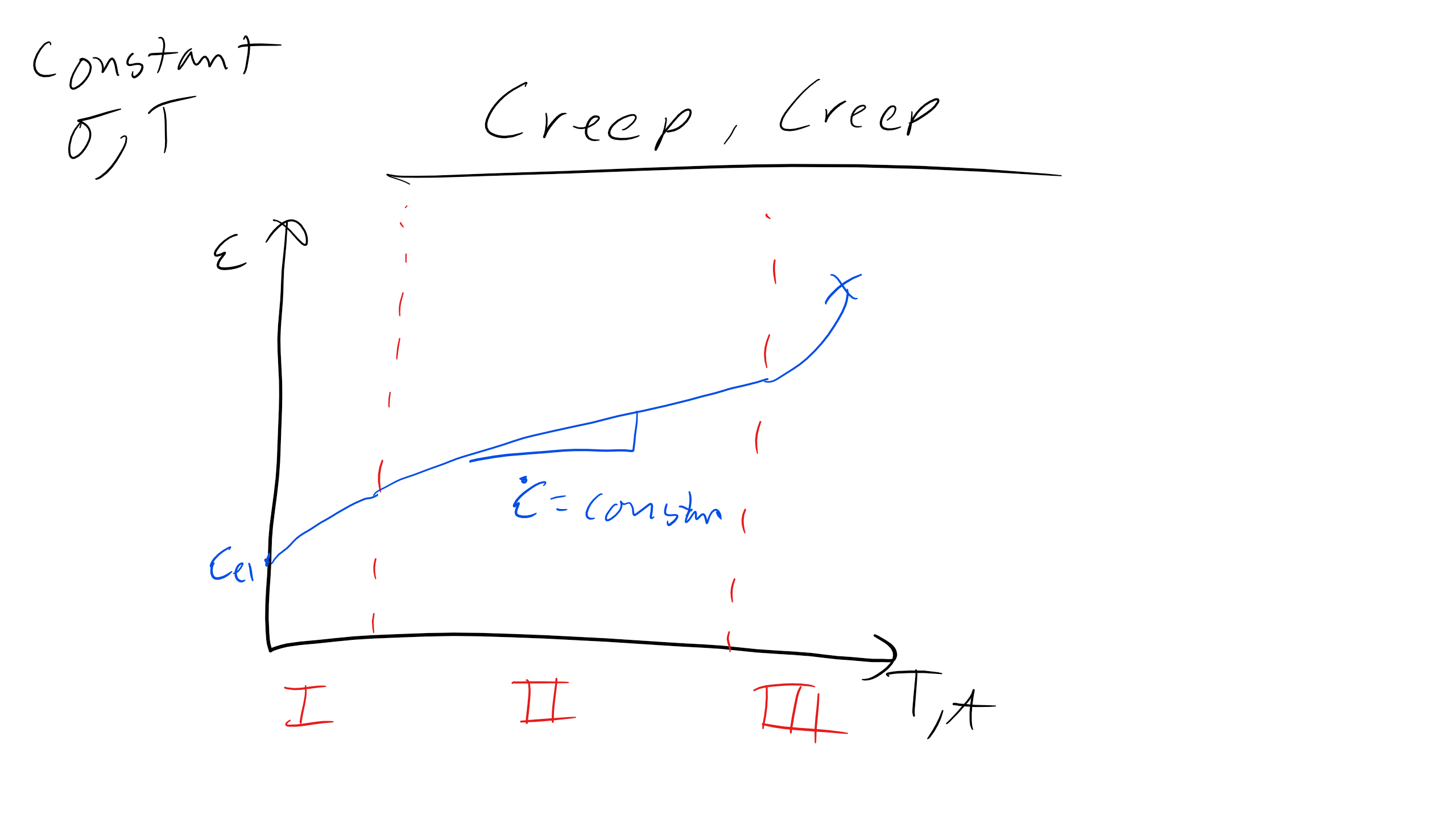
1. Primary or Transient Creep
2. Secondary or Steady State Creep
3. Tertiary or Runaway Creep

In the primary or transient creep regime the strain growth is relatively slow however once we reach the secondary creep regime we see the the strain grows at a constant strain rate \(\dot{\epsilon_c}\). This leads to large strains and can be a limiting factor in design. Now in the tertiary regime the strain increases extremely fast and this also known as runaway creep, no way to stop creep in this regime and it typically leads to failure. Creep is a critically important phenomenon in high temperature application like turbine blades, power stations, hot forming operations, and many others.

Again as materials scientists we want to focus on predicting the creep strain rate, \(\dot{\epsilon_{c}}\), so that we can determine the expected creep strain in our application and we can predict when the material may fail in an application. For example in an turbine engine we need to make sure the turbine blades to creep to an extent where they contact the turbine engine enclosure, that can be very bad!!

So when considering how we design applications to consider creep we have to ensure the following:

- The total creep strain is less than the allowable strain for a particular application
- The strain to failure must be greater than both the total creep strain and allowable strain for an application
- The time for the application must be less than the time to failure for creep

These may seem like obvious design criterion but both creep and fatigue are often the most overlooked phenomenon in application design and lead to most catastrophic failure in applications.

Now in addition to thermally activated diffusion we can also observe creep and diffusion that is driven by a mechanical force as well. Consider the following scenario if there is no applied force than in the image below atoms A and C are equally likely to diffuse into the vacancy B but if a material is loaded it is much more likely that A moves into B than C. Thus we have effectively introduced an energy potential into this system and thus biased the diffusion in a particular direction.

Let's talk about some more mechanisms in detail now to get an atomistic perspective before zooming out the macro scale.

Atomistic Mechanisms of Creep

Now before we get into our macroscopic view point and look at some beautiful equations and deformation mechanism maps let us consider creep at the atomistic length scale and one mechanism of how creep can occur is via diffusion. Now we have just had a thorough discussion of diffusion but we will see that several of the mechanisms of creep will occur via dislocation climb which is a thermally activated diffusion process. Now what is interesting in creep is that we are dealing with crystalline materials primarily when we discuss creep (creep also occurs in polymers which are viscoelastic materials but we can discuss creep in polymers more if people are interested) and there are actually multiple diffusive pathways in crystalline materials. Remember that most crystalline materials are poly-crystalline so there regions of perfect crystal which we will refer to as the bulk there are also multiple grain boundaries in polycrystalline materials and materials can also diffuse along grain boundaries as well as in or around other defects like dislocations, point defects, and even free surfaces. As we saw in our brief diffusion refresher typically atoms will diffuse faster when there is more available free space so atoms will diffuse faster in grain boundaries than in the bulk and this is because there is more open space and thus the activation energy for diffusion is lower in the grain boundaries than in the bulk \(Q_{GB}<Q_{B}\).

Bulk Diffusion

When we consider Bulk diffusion we will typically see atoms that move via vacancy diffusion into a site. Now there are other modes of diffusion where atoms can move into an interstitial site or a tetrahedral, octahedral, split-dumbell, and many other sites but for most metals, ionic crystals, and ceramics this is the most likely diffusion pathway.

Grain Boundary Diffusion

As we have mentioned previously grain boundaries meet when the crystal orientation is ofsett by some angle and as we discussed previously these can be high or low angles. In addition to this change in angle there will also typically be some width to the grain boundary and the structure will be more open than the rest of the crystal. Now typically this grain boundary width \(\delta\) will be at least two atomic diameters or around \(5\AA\) or very close to a \(nm\) so this distance is significant. Now at this point you may ask well if the grain boundary diffusion is so much faster than the bulk why are we even considering the contribution of the bulk? Well that is because even though the grain boundary diffusion is much faster its total contribution to creep depends on how much grain boundary is available to diffuse into and through so thus id depends on both the \(\delta\) and the grain diameter \(d_g\). We can actually compare the relative areas for grain boundary and bulk diffusion as follows we imagine a circular grain and let's neglect constants for now but for bulk diffusion the area will be approximately \(\bigg(\frac{d_g}{2}\bigg)^2\) whereas for a grain boundary it will be approximately \(\frac{\delta d_g}{2}\) so if we divide the area for grain boundary diffusion by that for bulk we get

\[
\frac{2\delta}{d_g}
\]

this is a very very important expression. We see that the relative areas depend inversely with grain size. The width of the grain boundary will not change appreciable but grain size can vary from 100s of \(\mu m\) to 10s of \(nm\) or less. That is a 4 order of magnitude change and it makes sense intuitively. As the grain size decreases due to conservation of volume there will be more crystalline grains and thus diffusion along grain boundaries will begin to dominate as there are more diffusive paths relative to large grain sizes and the enhanced diffusion will make this type of dislocation mechanism dominate the overall behavior. Vice versa can be said as grain size increases.

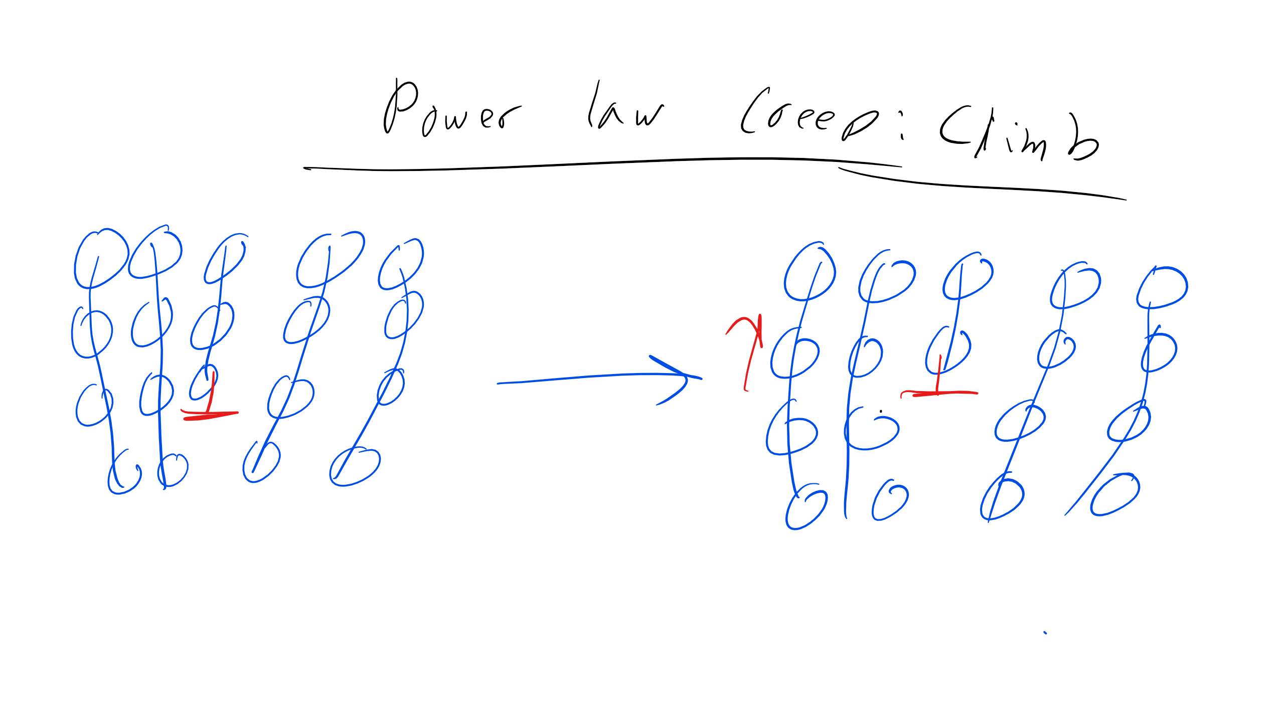
Power Law Creep Dislocation Climb

One more mechanism that we will delve into is just a bit is power law creep through dislocation climb. In this scenario there can be obstacles to dislocation climb i.e. point defects, precipitates, dislocations, which prevent or seriously inhibit dislocation glide. One method to move around these obstacles is for the dislocation to climb around the obstacles so the dislocation can continue to climb. This force can initiate the diffusion of atoms form the dislocation core as that is where stress is the largest. This process repeats to allow the dislocation to move through the material. Now remember that typically dislocation climb is a thermally activated process but we discussed previously that this assumption held for relatively small applied stresses. However, at high stresses this is not necessarily the case and as described above climb can be initiated.

General Creep Strain Rate Expression

Luckily we have developed a nice framework for describing creep in the secondary regime, we typically will neglect the first regime and once we reach the tertiary regime there is nothing we can do. So we can use the following general expression to describe the creep strain rate

\[
\dot{\epsilon_{c}} = K_{c} \sigma^{x} d^{y}_{g} D_{c} = K_{c} \sigma^{x} d^{y}_{g} D_{o} \exp\bigg(\frac{-Q_{c}}{kT}\bigg)
\]

where \(K_{c}\) is an empirical material specific creep constant, \(\sigma\) is the applied stress, \(d_{g}\) is the grain diameter, \(D_{c}\) is the creep diffusivity, and \(Q_{c}\) is the activation energy for that creep mechanism. Now those diffusion mechanisms are diffusion of vacancies through the lattice or bulk diffusivity, diffusion of vacancies along grain boundaries, and diffusion of vacancies to dislocations.

Lattice/Volume/Bulk Diffusion: Nabarro-Herring Creep

We have our equation for Nabarro-Herring Creep below:

\[
\dot{\epsilon_{NH}} = \frac{K_{NH}\sigma D_{o} \exp\bigg(\frac{-Q_{L}}{kT}\bigg)}{d^{2}_{g}}
\]

The key things to see in this equation is the activation energy for lattice diffusion and the scaling behavior with the grain size. Also note that this creep describes diffusion in the bulk and it is linear with stress. This mechanism will dominate at high temperatures, larger grain sizes, and intermediate to low stresses.

Grain Boundary Diffusion: Coble Creep

Here the number of diffusive pathways increases as the grain size decreases and remember that the activation energy for grain boundary diffusion is lower than for bulk.

\[
\dot{\epsilon_{CC}} = \frac{K_{CC}\sigma D_{o} \exp\bigg(\frac{-Q_{GB}}{kT}\bigg)}{d^{3}_{g}}
\]

The noticeable relationships here are that again we have a linear relationship with stress a strong dependence on grain size, even stronger that for NH creep. Also we see that the diffusion we describe here is grain boundary diffusion. Now this regime will get considerably larger and dominate when the grain size is small. Also this regime will tend to dominate at lower temperatures than NH creep. Why is this? Because remember the activation energy for diffusion in the grain boundary is lower than that for the bulk so we need less energy to get equivalently fast diffusion.

Power Law Creep

Here the net motion of dislocation cores moves in direction of applied stress, i.e. macroscopic creep. The dependence on applied stress is critical as you can see the scaling behavior in the equation below. Additionally dislocation climb is the rate-limiting process.

\[
\dot{\epsilon_{DLC}} = K_{NH}\sigma^{4-6} D_{o} \exp\bigg(\frac{-Q_{L}}{kT}\bigg)
\]

We can now take a look at some key aspects of creep and in particular the scaling behavior of creep:

\[
\begin {tabular} { | c | c | c | c | }
\hline
Mechanism & Q & x & y \\ \hline
NH & Q_{L} & 1 & -2\\ \hline
CC & Q_{GB} & 1 & -3 \\ \hline
PLC & Q_{L} & 4-6 & 0\\
\hline
\end {tabular}
\]

We can see that PLC will dominate at high temperatures and high stress and Coble creep will dominate at lower temperatures compared to NH.

You will notice that there are other distinct regions in this deformation mechanism map which shows the various mechanism of deformation. Note that on this plot the x-axis is a plot of the homologous temperature which is a dimensionless number which plots temperature divided by the melting temperature and we also have stress on the y-axis normalized by the shear modulus. In addition to our creep mechanisms we also have

- Theoretical Yield Strength: The dashed line is completely flat and indicates the theoretical yield strength of a material which is approximately \(\sigma_{theory} = \frac{G}{10}\). This line will never change location regardless of material.
- Elastic: Deformation that is purely elastic and dominates at low temperatures and stress, must be below the dislocation glide line which indicates the yield strength at different temperature conditions.
- Dislocation Glide: Deformation that is plastic and deformation occurs exclusively through dislocation glide. The stress is above the yield stress of the material which is indicated by the solid black line.

One of the ways to mitigate or prevent creep is typically close packed structures are more creep resistant also if one solute strengthens, precipitate strengthens, or increasing grain size as it slows creep due to fewer diffusive pathways along grain boundaries. Superalloys typically leverage this technique through the precipitating strengthening and anti-phase boundaries (APB). Also many high temperature applications will even use single crystal materials to avoid CC creep.

Fracture Regime

Finally Fracture!!

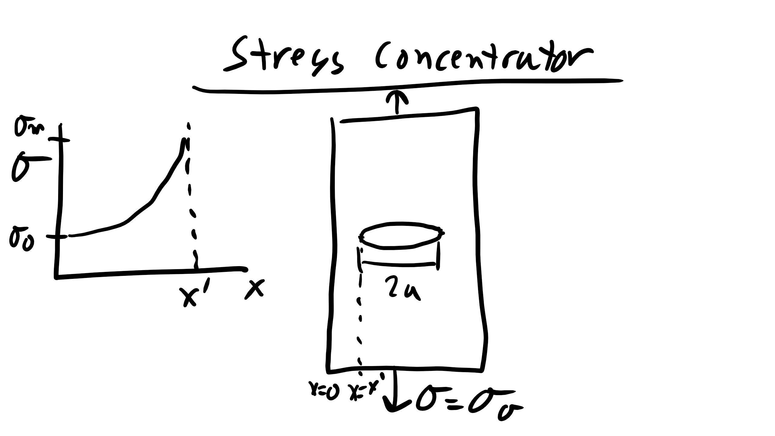
Fracture is the last resort for material deformation mechanisms when all other elastic/plastic mechanisms are exhausted. Energy is dissipated by bond breaking. In uniaxial loading, the stress required to break the material in two pieces, at the stress fracture. Again as in the case of yielding the theoretical stress required to fracture materials (Steel 4340 65GPa, Al 20GPa, Si 7GPa) is orders of magnitude higher than the actual stress required to fracture materials (Steel 4340 ~3GPa, Al ~0.7GPa, Si ~0.3GPa). This is because real materials typically contain cracks (inside, at surface, or at interfaces) and these micro-cracks act as stress concentrators. For an elliptical hole we can define the stress as a function of the distance from the stress concentrator as:

\[
\sigma = \sigma_{o}\bigg(1+2\sqrt{\frac{a}{R}}\bigg)
\]

and R at the tip of the crack is \(\frac{b^2}{a}\). Brittle fracture occurs when the stress concentration at a pre-existing crack tip is so high that the material will break catastrophically.

Griffith's Theory of Brittle Fracture

We can develop an equation for brittle fracture from Griffith by considering the surface area created as the crack grows and the stored elastic energy that is relieved. Note that this derivation is particularly valid for very brittle materials like glasses and ceramics.

When considering fracture, the two energy contributions are: creating surface area (energy penalty) and relieving elastic strain energy (energy release). Creating surface area results in a positive energy contribution that resists crack growth, while relieving strain energy provides a negative contribution that drives crack propagation. Fracture will proceed when the reduction in elastic strain energy equals or exceeds the energy required to create new surfaces.

Relieving Stored Elastic Energy

We know that we can calculate the stored elastic strain energy in a material as:

\[
U_{ESE} = \int \sigma d\epsilon = \frac{\sigma^2}{2E}
\]

Note here that we are assuming the material is very brittle, so \(\sigma = E\epsilon\). This is the energy per unit volume, so to obtain the total energy, we multiply by the volume of the elliptical crack, approximated as:

\[
\Delta U_{el} = -\frac{\pi a^{2} t \sigma^{2}}{2E}
\]

The negative sign indicates that this term represents a reduction in energy as the crack grows.

Creating Surface Area as Crack Grows

When a crack grows, two new surfaces are created, with a total area approximated as:

\[
\Delta U_{surf} = 4at\gamma
\]

Now the crack reaches its critical length when the total energy is minimized:

\[
\Delta U_{tot} = \Delta U_{surf} + \Delta U_{el} = 0
\]

This gives us Griffith’s expression for the critical stress for fracture:

\[
\sigma_{f} = \sqrt{\frac{2 \gamma E}{\pi a_{crit}}}
\]

Note that this derivation assumes the stress is constant at the crack tip, which is an approximation.

Orowan Theory of Ductile Fracture

There are a number of materials, metals and polymers, which will not fracture in a completely brittle manner but instead through the formation of a small plastic zone prior to each crack elongation. For these materials, Orowan proposed a theory for ductile fracture:

\[
\sigma_{f} = \sqrt{\frac{E G_{c}}{\pi a}}
\]

where \(G_{c}\) is the strain energy release rate.

Stress Intensity Fracture and Fracture Toughness

We can relate the Griffith criterion for fracture to useful material parameters such as the stress intensity factor and fracture toughness.

Rewriting Griffith’s equation:

\[
\sigma \sqrt{\pi a} = \sqrt{2 \gamma E}
\]

The left-hand side represents the applied conditions (loading), and the right-hand side represents material properties. We define the stress intensity factor as:

\[
K_I = f \sigma \sqrt{\pi a}
\]

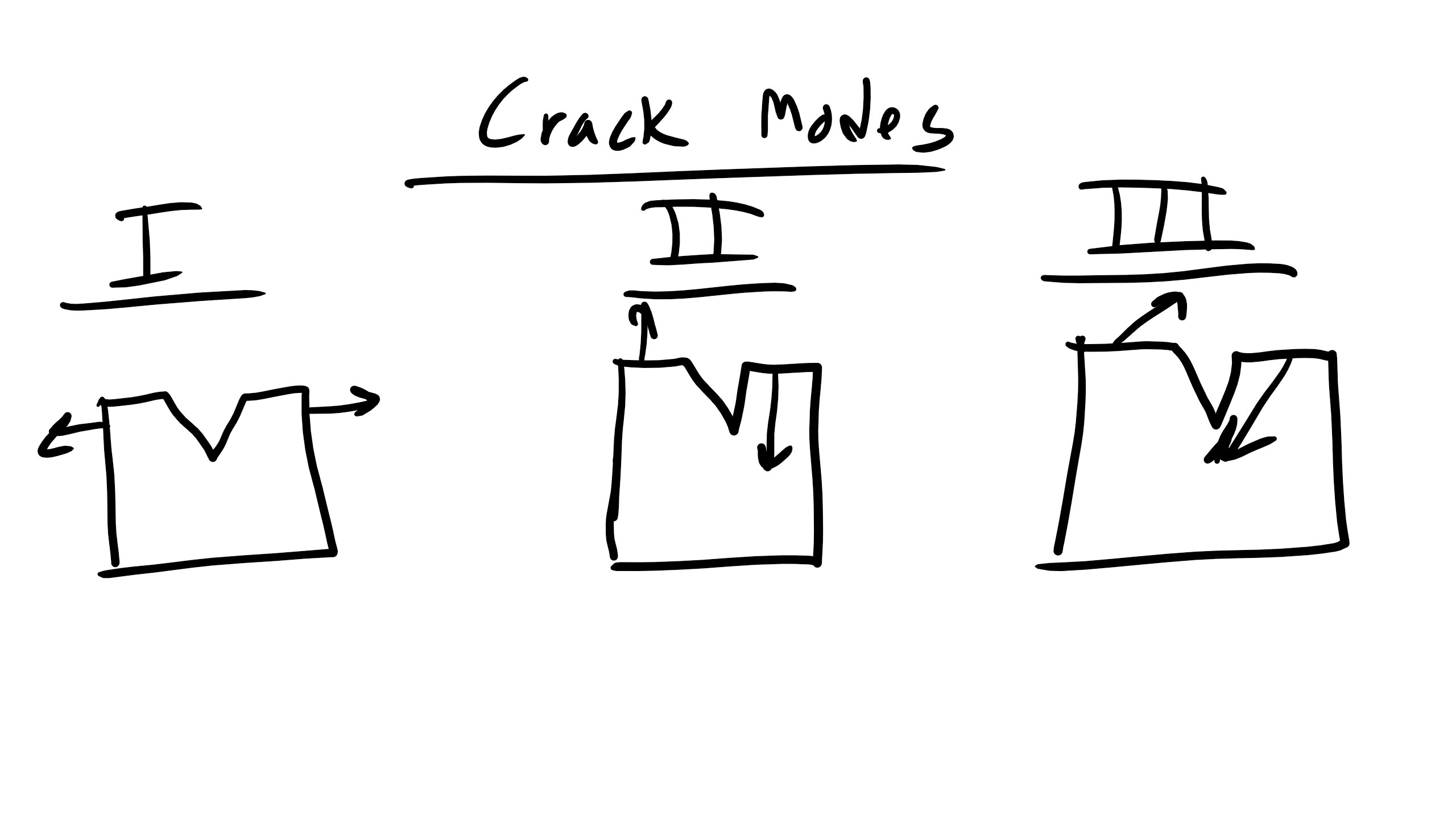
where \(f\) is a geometric correction factor. The subscript “I” indicates the fracture mode (Mode I: opening mode). Modes II and III correspond to in-plane shear and out-of-plane shear, respectively.

The fracture toughness is defined as a material property:

\[
K_{IC} = \sqrt{E G_c}
\]

with units of Pa\(\sqrt{m}\). Fracture occurs when:

\[
K_I = K_{IC}
\]

If \(K_I < K_{IC}\), the material will not fracture. This criterion can also be used to determine the critical crack length or the stress required for fracture.

Now, we previously mentioned that a plastic zone develops near the crack tip. Because the stress at the crack tip theoretically approaches infinity, a small region undergoes yielding, forming a plastic zone of radius \(r_p\).

The Griffith equation is only valid when this plastic zone is small, specifically when:

\[
\frac{r_p}{a} < 0.02
\]

If this condition is not met, the Griffith approach cannot be used.

To estimate \(r_p\), we assume a plane stress condition. The local stress field near the crack tip can be approximated by:

\[
\sigma_{local} \approx \frac{\sigma \sqrt{\pi a}}{2 \pi r} \approx \frac{K_I}{2 \pi r}
\]

Equating this to the yield stress gives:

\[
\sigma_{y} = \frac{K_I}{\sqrt{2 \pi r_p}} = \frac{\sigma \sqrt{\pi a}}{\sqrt{2 \pi r}}
\]

Thus, the plastic zone size is:

\[
r_p = \frac{K^2_I}{2 \pi \sigma^2_y}
\]

This provides a good approximation for many materials.

Mechanisms of Fracture

Typically when we want to obtain a physical understanding of fracture we must understand that fracture is somewhat stochastic in that cracks will typically initiate where stress is concentrated the most, typically at microcracks, and these cracks are distributed stochastically and will propagate in a manner that follows the lowest energy path, i.e. to relieve elastic strain energy the most.

For ceramics and glasses, which are very brittle, cracks will propagate quite easily with minimal plastic deformation. Additionally, the fracture surface of these materials will be quite smooth and flat, again exhibiting little to no plastic deformation. This flat surface comes from the cleaving of atomic planes.

Most metals will typically fracture in a ductile manner and will have some plastic zone, but at certain temperature conditions may fracture in a brittle manner. The fracture surface for ductile metals will be much more rough due to this plastic deformation, and as you may imagine, materials with a larger yield strength will typically have a smaller plastic zone, whereas materials that exhibit a smaller yield stress will have a larger plastic zone.

Fracture for ductile metals often starts near inclusions within a metal, which are chemical compounds where the metal reacts with impurity atoms; this is a large problem in industry. The plastic flow typically will take place around these inclusions, leading to elongated cavities that line up and turn a sharp crack into a blunt one. Blunting a crack tip is the key to obtaining high toughness, and the ability of these inclusions to blunt crack propagation is important.

Polymers are much more complicated and can fracture in a ductile or brittle manner depending on temperature, time, and strain rates. Also, the toughness of these materials can increase by including rubber precipitates or by developing composites which blunt crack propagation.

Ductile to Brittle Transitions

Often metals and other materials can exhibit a ductile to brittle transition, and this transition depends on several parameters, specifically the yield stress and the size of the plastic zone.

Additionally, the yield stress also depends on temperature and strain rate as described by the following expression:

\[
\sigma_y = \sigma^o_y \bigg( 1- \frac{kT}{Q_b} \ln \frac{\dot{\gamma}}{\dot{\gamma_o}}\bigg)
\]

where \(\sigma^o_y\) is the yield strength at \(0K\), \(Q_b\) is the energy per bond, \(\dot{\gamma}\) is the shear strain rate, and \(\dot{\gamma_o}\) is a material parameter.

Additionally, remember that we have:

\[
r_p \approx \bigg( \frac{K_I}{\sigma_y}\bigg)^2
\]

These expressions lead us to the following general relationships that are somewhat intuitive: as temperature decreases, the yield strength increases and plastic zone size decreases, thus the material becomes more brittle. Equivalently, the same occurs as the strain rate increases. This highlights a very important relationship — Time-Temperature Equivalence. This ductile-to-brittle transition is most notably observed as the cause for the fracture of liberty ships during World War II.

Creep Fracture

Fracture can also occur as a result of secondary creep and tertiary creep. Creep fracture typically occurs intergranularly, i.e. along the grain boundaries as opposed to trans- or intragranularly. The way that creep fracture occurs is via the coalescence of voids due to diffusion of material away from the grain boundaries, i.e. vacancies left behind as material moves along grain boundaries. This eventually causes rupture and can be described by some empirical relationships, specifically the Monkman-Grant equation and/or the Larson-Miller parameter.

Increasing Toughness by Blunting Crack Tip Propagation

There are multiple ways to increase the toughness of a material and reduce brittle fracture. One of the ways this is done in polymer blends is by including rubbery or soft inclusions, by blending a brittle polymer with a more rubbery polymer. This is most noticeable in High Impact Polystyrene (HIPS), where we blend polystyrene (PS) with a rubbery polymer, polybutadiene (PB), in order to increase the toughness of the material while paying a cost in stiffness.

We can also create self-healing materials which seek to heal cracks and close them as they propagate. This is commonly done with microcapsules that activate an epoxy or a chemical reaction which fuses the crack. Additionally, depending on the diffusivity of the material, some can actually self-heal via diffusion.

Composites are also excellent examples of methods to increase the toughness of materials as they are typically composed of a brittle and more ductile component. Even if the composite is made of two brittle components, as the crack interacts with the different component it tends to be blunted and stops propagating.

Fatigue

Fatigue (cyclic) loading occurs at applied stresses that are much lower than the stress at fracture or even the yield stress but again, like creep, can lead to catastrophic failure at these low applied stresses.

Fatigue can occur in components or applications where there is no pre-existing crack and it can also occur where there is a pre-existing crack. Now typically most materials will have some pre-existing or microcracks, but there are certain applications like small components such as gear teeth where there may not be significant microcracks.

Let's consider the scenario where there are no pre-existing cracks first.

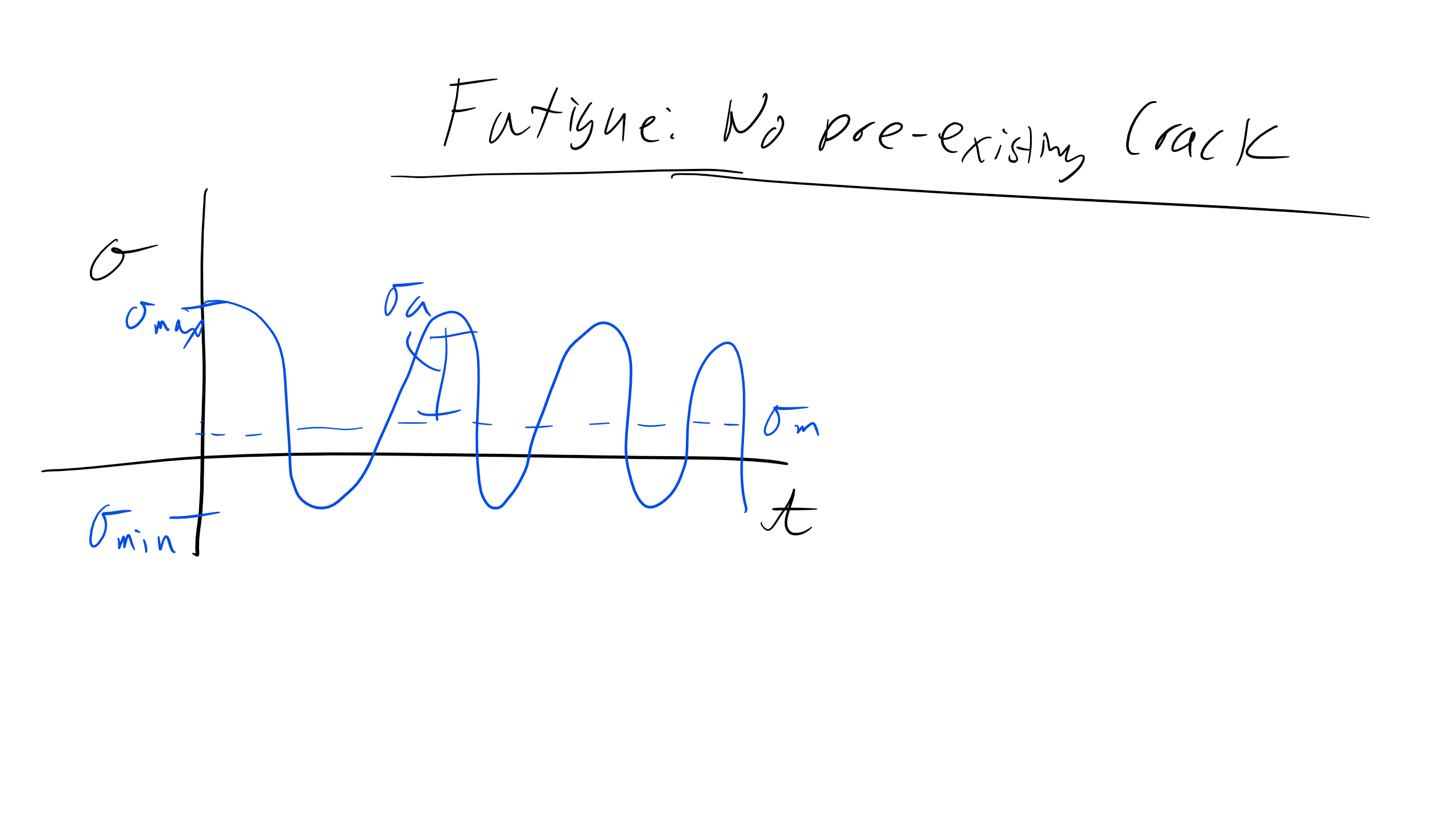
Fatigue: No Pre-existing Cracks

With a fatigue-type loading scenario, we will assume some type of cyclical loading with a particular number of cycles \(N\), a number of cycles to failure \(N_F\), and a maximum stress \(\sigma_{max}\), and minimum stress \(\sigma_{min}\) as seen below.

Note that the change in stress is described as \(\Delta \sigma = \sigma_{max} - \sigma_{min}\) and the mean stress is described as \(\sigma_m = \frac{\Delta \sigma}{2}\).

For systems that have no pre-existing cracks we can describe the fatigue in two regimes: low-cycle and high-cycle fatigue. Typically, low-cycle fatigue will fail at fewer than \(10^4\) cycles and high-cycle fatigue will fail at more than \(10^4\) cycles.

We can actually develop a relationship that describes the change in stress to the number of cycles to failure as follows for high-cycle fatigue, and this is known as Basquin’s Law:

\[
\Delta \sigma N^a_f = C_1
\]

where \(a\) and \(C_1\) are material properties and typically \(\frac{1}{15}<a<\frac{1}{8}\). The low-cycle fatigue instead relates the change in plastic strain to the number of cycles to failure as described by the Coffin-Manson law:

\[
\Delta \epsilon^{pl} N^b_F = C_2
\]

where \(b\) will typically vary from 0.5–0.6.

Also, if \(\Delta \sigma\) varies over the lifetime we can apply Miner’s rule of cumulative damage to determine when the number of cycles to failure has been met using the following relationship:

\[
\Sigma \frac{N_i}{N_{f,i}} = 1
\]

where \(N_{f,i}\) is the number of cycles to fracture for each region \(i\), and the ratio represents the fraction of lifetime used up after \(N_i\) cycles in that region.

Fatigue with Pre-Existing Cracks

The more common scenario you will most likely encounter is when we work with fatigue for a material that has pre-existing cracks. First you may be asking how can we tell if a material has pre-existing cracks? Well, have you ever seen people at the airport with a handheld device pressed near the exterior of the plane?

Those people are non-destructively looking for the presence of micro-cracks using ultrasound. You can also use X-rays for this, but using these techniques we can measure the distribution of crack sizes in a material and then use the following formalism to determine the number of cycles to failure for an initial crack length.

Fatigue failure is fracture due to crack growth every cycle of loading or the crack growth increment per loading cycle, defined below:

\[
\frac{da}{dn}
\]

where \(a\) is the crack length and \(n\) is the number of loading cycles.

We will deal with Static Fatigue and Cyclic or Classical Fatigue. Static fatigue occurs when a material is placed under a static or constant load and the crack faces of a material interact with the environment. The crack tip becomes embrittled due to interaction with the environment (stress corrosion cracking), the crack tip sharpens, the crack propagates, and the process repeats.

The more common fatigue scenario is cyclic or classical fatigue, where a material is under a cyclic load or stress. We need to define the cyclic applied stress, specifically the frequency of the applied load, \(f\), which is \(\frac{1}{\tau}\), where \(\tau\) is the period of the applied stress. We also want to quantify the stress ratio, \(R\):

\[
R = \frac{\sigma_{min}}{\sigma_{max}}
\]

As materials scientists we want to avoid catastrophic failure, and for fatigue that involves trying to estimate the number of cycles to failure, \(N_{f}\), which is the number of cycles to grow a crack from initial length \(a_{o}\) to the critical or catastrophic crack length \(a_{c}\).

There are three distinct regimes of fatigue crack growth: I) The Slow-Growth Rate or Near-Threshold Regime, II) Mid-Growth Rate or the Paris Regime, and III) High-Growth Rate Regime.

I) Slow-Growth Rate or Near-Threshold Regime

In the slow-growth rate regime the crack won’t grow initially until the threshold stress intensity factor, \(\Delta K_{th}\), is reached where:

\[
\Delta K = f \Delta \sigma \sqrt{\pi a}
\]

Typically we say that when the rate of crack growth is \(10^{-8}\) mm/cycle or less, the crack is dormant or growing at a near-undetectable rate. Once the threshold stress intensity factor is reached, the crack growth rate will increase but still the growth rate is extremely slow, still below one lattice spacing per cycle, until we reach the Mid-Growth Rate or the Paris Regime.

II) Mid-Growth Rate or Paris Regime

In the Mid-Growth Rate or Paris Regime we actually have an equation or law to describe fatigue crack growth, aptly named the Paris Law:

\[
\frac{da}{dN} = C\Delta K^{m}
\]

where \(C\) and \(m\) are empirical constants which depend on the material, the applied stress, frequency, and \(R\). Typically for metals \(m\) will approach 3 or 4.

We can use the Paris Law to predict the number of cycles to failure, \(N_{f}\):

\[
\int^{N_{F}}_{0}dN = \int^{a_{c}}_{a_{o}} \frac{da}{C(f \Delta \sigma \sqrt{\pi a})^m}
\]

which leads to:

\[
N_{f} = \frac{1}{C(f \Delta \sigma \sqrt{\pi})^m} \bigg[\frac{a^{1-\frac{m}{2}}_{c} - a^{1-\frac{m}{2}}_{o}}{1- \frac{m}{2}}\bigg]
\]

Fatigue cracks are marked via striations on the fracture surface.

III) High-Growth Rate Regime

The last stage, the high-growth rate regime, is characterized by an orders-of-magnitude increase in the crack growth rate and additional cleavage in the material or microvoid coalescence. This is the end region where catastrophic crack failure will occur throughout the material. We need to take the material out of service before we reach this regime.

One way that we can try to predict the lifetime of materials is by looking at empirically determined S-N curves. \(S\) is the stress amplitude (the difference between the maximum and minimum applied stress). \(N\) is again the number of cycles. We can look at the curve and determine when the material will fail.