Chapter 9: Plasticity Regime

Plasticity Regime

In the plastic regime, we have discussed previously that deformation is permanent and irreversible. Additionally, unlike in the elastic regime where we spend a considerable amount of time deriving and developing constitutive equations that relate stress to strain, in the plastic regime we will not have such relationships. Instead, we will develop our understanding of the mechanical behavior of materials from an empirical, evidence-based perspective.

Some materials, like ceramics, exhibit very little to no plasticity and tend to fracture before yielding occurs. Additionally, in this lecture we will only discuss low-temperature plasticity — i.e. at temperatures below those where creep can be activated. (Creep will be discussed in a subsequent lecture.) For metals, the temperature for creep to occur is typically \( \frac{T}{T_m} > 0.3 \) and for ceramics \( \frac{T}{T_m} > 0.5 \).

One of the critical parameters that defines plasticity and dominates our discussion is the yield strength. The yield strength can be measured in several different ways:

- Uniaxial Tension Testing
- Hardness Testing
- Nanoindentation

Before we get too deep into plasticity, let's start with a fun calculation of what should be the theoretical yield strength of a material to highlight a critical aspect of materials science — that defects are essential to determining mechanical behavior.

Theoretical Yield Strength of Materials

We have previously shown that by taking an atomistic perspective we were able to develop a good approximation of the stiffness of a material from first principles. Let’s attempt a similar approach for yielding.

Consider a perfect crystal subjected to a shear stress. For yielding to occur, atoms must slide over one atomic spacing.

If we consider the forces required to do so, we must consider the bond energy function, as discussed previously when deriving the Young’s modulus. We can approximate this force function using a harmonic expression:

\[
\tau = \tau_{max} \sin\left(2\pi \frac{x}{a}\right)
\]

where \( a \) is the interatomic spacing, typically \( 2R \). The engineering shear strain is then:

\[
\gamma = \frac{x}{a}
\]

We can relate \( \tau_{max} \) to the shear modulus \( G \) as follows:

\[
\frac{d\tau}{d\gamma} = \frac{d\tau}{dx}\frac{dx}{d\gamma} = a \tau_{max} \frac{2\pi}{a} \cos\left(\frac{2\pi}{a}\right)
\]
\[
G = \left(\frac{d\tau}{d\gamma}\right)_{\gamma \to 0} = 2\pi \tau_{max}
\]

Thus, the material should yield at a stress of approximately:

\[
\tau_{yield} = \frac{G}{2\pi} \approx \frac{G}{10}
\]

For most materials, this would predict a yield strength of about 10 GPa, yet experimental yield stresses are typically only 10–100 MPa — about three orders of magnitude smaller. Why?

Even with more accurate potential models, the theoretical prediction still does not match experimental results. The answer lies in a subtle but profound realization that defects control plasticity. This realization led to one of the most significant theories in materials science: Dislocation Theory.

Dislocation Theory

Before we get deep into dislocation theory, let’s recall some of our old friends: edge dislocations, screw dislocations, point defects, and grain boundaries. This is where all those concepts come together.

Historically, the question of why the theoretical yield strength was so much higher than the experimental value was answered independently by Taylor, Polanyi, and Orowan. They proposed that we do not have to slip entire planes of atoms simultaneously — which would require breaking all bonds in a plane — but instead, a few or even one bond at a time can move.

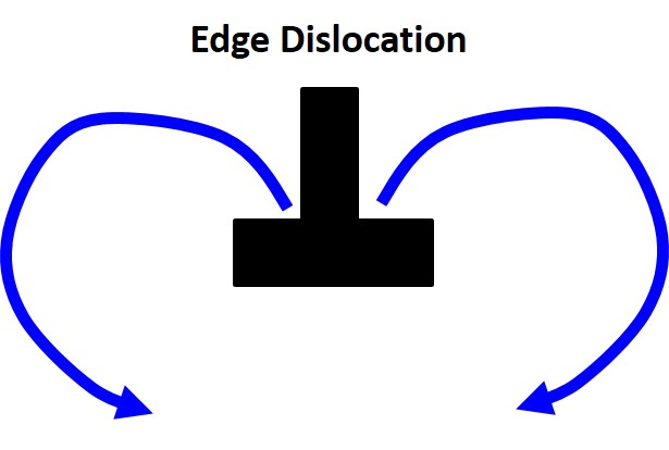
To visualize this, imagine an inchworm moving along a surface. In effect, a single extra half-plane of atoms moves incrementally from its equilibrium position to a new position halfway between atomic planes, creating an edge dislocation in the process.

A dislocation produces a local stress/strain field in the crystal lattice. Specifically, at the top of the dislocation, atoms are compressed relative to their equilibrium positions, while below the dislocation there is a tensile region where smaller atoms can diffuse. The amount of atomic displacement or distortion depends on bond stiffness. The interplanar spacing between close-packed planes is greater for FCC than for BCC structures, leading to larger distortions in FCC materials. The dislocation width is smaller in ionically bonded ceramics and even smaller in covalently bonded materials due to their higher bond stiffness.

Intuitively, a dislocation can move much more easily than an entire slip plane, since only a small number of bonds need to be broken sequentially. This motion of dislocations is referred to as slip, and whether a material can slip depends on several factors.

However, dislocations are not entirely free to move without resistance. When a dislocation moves, it drags along regions of compressive and tensile distortion, which create local strain fields that resist motion. This resistance is referred to as the Peierls force, and it depends on the crystal type, temperature, and other factors. Generally, materials with wide dislocations have a lower Peierls force. Hence, this force is smaller for FCC materials than BCC materials, and smaller for metals than ceramics. The Peierls force also decreases with temperature since dislocation motion becomes thermally activated.

Dislocation Stress Fields

We can describe the stress field associated with an edge or screw dislocation for isotropic, linear elastic materials. Consider an infinite edge dislocation along the z-axis with a Burgers vector along the x-axis. The stress field is given by:

\[
\sigma_{xx} = -Dy \frac{3x^2 + y^2}{(x^2 + y^2)^2}
\]
\[
\sigma_{yy} = Dy \frac{x^2 - y^2}{(x^2 + y^2)^2}
\]
\[
\sigma_{xy} = Dx \frac{x^2 - y^2}{(x^2 + y^2)^2}
\]
\[
\sigma_{zz} = \nu (\sigma_{xx} + \sigma_{yy})
\]
\[
D = \frac{G b}{2\pi(1 - \nu)}
\]

All other stress components are zero.

For a screw dislocation, the displacement field can be described as follows. If we take a circular path around the dislocation, we find that \( u_x = u_y = 0 \) and \( u_z = b \). The displacement can be expressed as:

\[
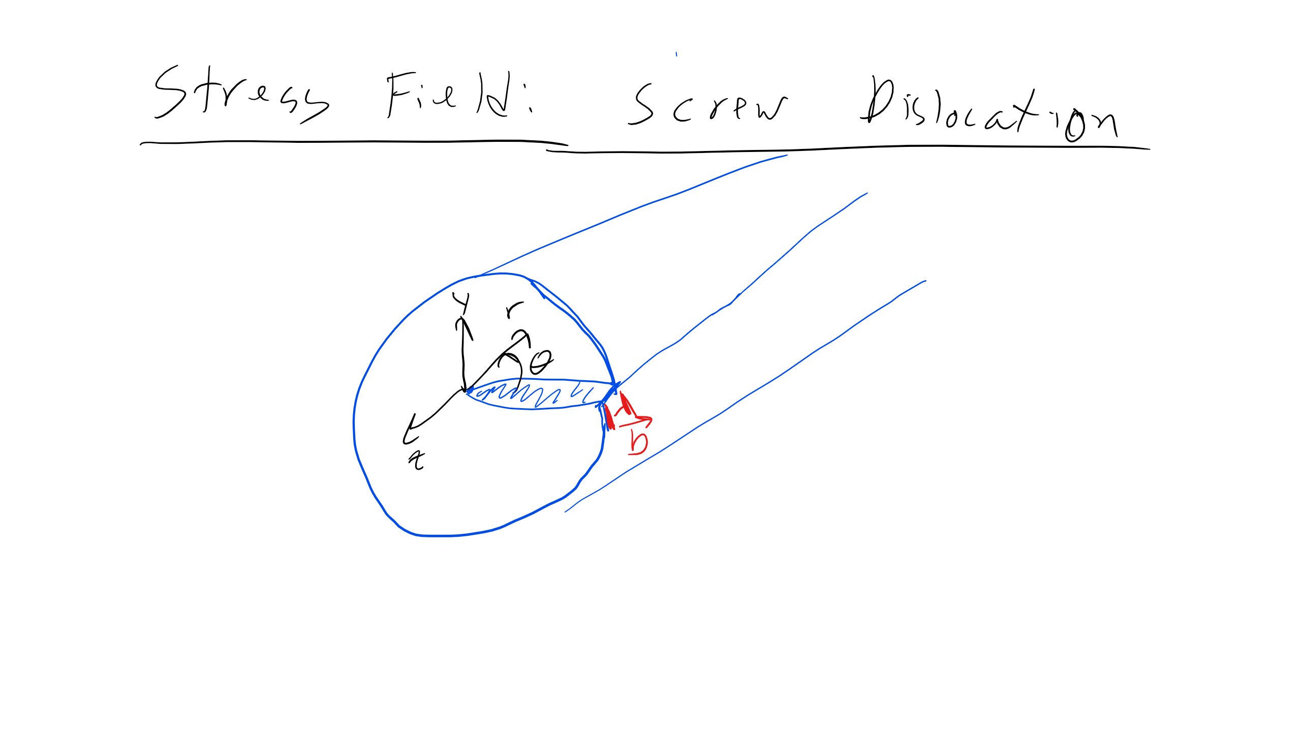
u_z = \frac{b \theta}{2\pi} = \frac{b}{2\pi} \tan^{-1}\left(\frac{y}{x}\right)
\]

The normal strains are all zero:

\[
\epsilon_{xx} = \frac{\partial u_x}{\partial x} = \epsilon_{yy} = \frac{\partial u_y}{\partial y} = \epsilon_{zz} = \frac{\partial u_z}{\partial z} = 0
\]

The shear strains are:

\[
\gamma_{xy} = \frac{\partial u_x}{\partial y} + \frac{\partial u_y}{\partial x} = 0
\]
\[
\gamma_{yz} = \frac{\partial u_y}{\partial z} + \frac{\partial u_z}{\partial y} = \frac{b x}{2\pi(x^2 + y^2)}
\]
\[
\gamma_{xz} = \frac{\partial u_z}{\partial x} + \frac{\partial u_x}{\partial z} = \frac{-b y}{2\pi(x^2 + y^2)}
\]

The corresponding stresses are:

\[
\sigma_{xz} = -\frac{G b y}{2\pi(x^2 + y^2)}
\]
\[
\sigma_{yz} = \frac{G b x}{2\pi(x^2 + y^2)}
\]

All other stress components are zero.

These equations were first derived in 1905, long before the modern understanding of dislocations and their stress fields. A few key observations can be made:

- The stress is proportional to the Burgers vector and the shear modulus.
- There is a singularity at the dislocation core where linear elasticity breaks down.
- Screw dislocations produce pure shear stress.
- Edge dislocations produce both normal and shear stresses, resulting in compression above and tension below the slip plane.

The presence of normal stresses in edge dislocations enables strong interactions with point defects, as we will discuss next.

Dislocation Energy

Now that we know the stress fields generated by edge and screw dislocations, we can calculate their corresponding elastic strain energy. Let’s begin with a screw dislocation, using cylindrical coordinates for simplicity. For a screw dislocation, we can write the stress as:

\[
\sigma_{\theta z} = \frac{G b}{2 \pi r}
\]

The associated shear strain is:

\[
\gamma_{\theta z} = \frac{b}{2 \pi r}
\]

The elastic strain energy per unit volume is then:

\[
U_{screw} = \int_V \frac{1}{2}\sigma_{\theta z}\gamma_{\theta z} dV
\]

Substituting, we find:

\[
U_{screw} = \int_V \frac{G b^2}{8 \pi^2 r^2} dV = l \int_{r_0}^{r} \frac{G b^2}{8 \pi^2 r^2} 2 \pi r dr
\]

Since a dislocation is a one-dimensional defect, we usually express the energy per unit length:

\[
\frac{U_{screw}}{l} = \frac{G b^2}{4\pi} \ln\left(\frac{r}{r_0}\right)
\]

A similar expression can be derived for an edge dislocation:

\[
\frac{U_{edge}}{l} = \frac{G b^2}{4\pi(1 - \nu)} \ln\left(\frac{r}{r_0}\right)
\]

Important observations:

- The energy scales with \( G b^2 \).
- The energy diverges logarithmically as the radius increases, indicating that isolated dislocations have very high energy.
- Dislocations tend to move toward free surfaces or combine destructively with other dislocations to reduce their strain energy.

Dislocation Interactions with Point Defects

Dislocations can also interact with point defects. When a vacancy forms in a crystal, the surrounding atoms relax inward, resulting in a negative relaxation volume \( \Delta v_v \). For an interstitial atom, relaxation is outward, producing a positive relaxation volume \( \Delta v_i \). These relaxation volumes interact with the hydrostatic pressure in the crystal, defined as:

\[
p = -\sigma_{hydrostatic} = \frac{-1}{3}(\sigma_{11} + \sigma_{22} + \sigma_{33})
\]

This interaction modifies the formation energy of the defect:

\[
\Delta H^{f'}_x = \Delta H^f_x + p \Delta v_x
\]

If the internal pressure is positive, the formation energy of a vacancy decreases (making it easier to form), while the formation energy of an interstitial increases.

Screw dislocations, which are pure shear defects, do not have hydrostatic pressure components and thus do not significantly interact with point defects. Edge dislocations, however, have both tensile and compressive regions, leading to strong interactions.

At the top of an edge dislocation (compressive region, \( p > 0 \)), vacancies are attracted. Below the dislocation (tensile region, \( p < 0 \)), interstitials are attracted. Since interstitials produce larger volume changes than vacancies, their driving force for diffusion is correspondingly stronger. This explains the formation of defect atmospheres — such as Cottrell atmospheres — where solute atoms segregate to dislocations and pin them in place.

Mechanical Forces on Dislocations

Let’s now consider the mechanical forces acting on dislocations. Imagine a solid under a shear stress \( \sigma_{31} \) and assume that the solid is a cube with dimensions \( l_1, l_2, l_3 \).

As shown, a screw dislocation nucleates and moves, leaving behind a step one Burgers vector in height as it passes through the crystal. The Burgers vector is always parallel to the direction of slip motion — the direction in which the dislocation moves.

The work done on the body by the applied shear stress is:

\[
\Delta W = \sigma_{31} l_1 l_2 b
\]

Alternatively, we can consider the work done as the product of force per unit length \( f \) and the distance moved by the dislocation over the area \( l_1 l_2 \):

\[
\Delta W = f l_1 l_2
\]

Equating these expressions gives the force per unit length exerted by the applied stress on the dislocation:

\[
f = \sigma_{31} b
\]

A similar expression can be derived for edge dislocations. This force can also be derived from the gradient of the strain energy per unit length:

\[
f = -\frac{\partial (U/l)}{\partial d}
\]

where \( d \) is the dislocation displacement. The strain energy decreases as the dislocation moves toward a free surface — a key driving force for recovery and annealing processes.

Peach–Koehler Force

To generalize the dislocation force, consider a dislocation with Burgers vector \( \overline{b} \), line direction \( \overline{t} \), and an external stress tensor \( \sigma \). If the dislocation moves an infinitesimal distance \( ds \) in direction \( \overline{e} \), the work done is:

\[
dW = -\overline{b} \cdot [\sigma (\overline{t} \times \overline{e})] ds
\]

The force per unit length on the dislocation is then:

\[
\overline{f} = -\frac{dW}{ds} = \overline{e} \, [(\sigma \overline{b}) \times \overline{t}]
\]

or equivalently,

\[
\overline{f_{PK}} = (\sigma \overline{b}) \times \overline{t}
\]

This is the Peach–Koehler force, which describes the mechanical force acting on a dislocation line in any stress field. It is important to emphasize that the force arises from the external stress field, not from the dislocation’s own stress. The applied stress can come from other dislocations, grain boundaries, or external loading.

This derivation is a remarkable result — we have derived a force at the defect level using continuum mechanics and energy concepts. This multiscale linkage between atomic and macroscopic behavior is a hallmark of materials science. Importantly, the Peach–Koehler force represents a thermodynamic driving force (derived from energy gradients), not a classical Newtonian force.

Dislocation Glide and Climb

The Peach–Koehler force provides the driving force for dislocation motion. When the force acts within the dislocation’s slip plane, it causes glide. Glide occurs when shear stress is applied along the slip plane, allowing the dislocation to move through the crystal lattice and produce plastic deformation. The dislocation moves in the plane that contains both its line direction and Burgers vector.

Dislocation climb, on the other hand, involves motion perpendicular to the slip plane. Climb requires the diffusion of vacancies or atoms to or from the dislocation core and is therefore a thermally activated process. Climb is crucial for high-temperature deformation mechanisms such as creep.

Mixed dislocations, which have both edge and screw components, can experience both glide and climb, depending on local stress and temperature conditions.

Diffusion in Materials Refresher

Before continuing our discussion of dislocation motion, it is useful to review the fundamental principles of diffusion, as diffusion is essential for dislocation climb and other thermally activated processes.

Thermodynamics is the study of equilibrium states, where the state variables of a system do not change with time. Kinetics, in contrast, is the study of the rates at which systems that are out of equilibrium evolve toward equilibrium under the influence of various driving forces.

Diffusion and Fick’s First Law

Diffusion is the phenomenon of material transport by atomic motion. It typically involves the flux of chemical components, which arises from gradients in driving forces such as electrostatic potential, stress, temperature, or chemical potential.

Fick’s First Law expresses diffusion due to a concentration gradient:

\[
\vec{J_i} = -D \nabla c_i = -D \frac{\partial c_i}{\partial x}
\]

where:
- \( D \) is the diffusion coefficient (mass diffusivity),
- \( \vec{J_i} \) is the flux of species \( i \),
- \( \nabla c_i \) is the concentration gradient.

This equation has the same mathematical form as other transport laws. For example, in heat transfer:

\[
\vec{J_Q} = -k \nabla T
\]

where \( \vec{J_Q} \) is the heat flux, \( k \) is the thermal conductivity, and \( \nabla T \) is the temperature gradient.

Similarly, for charge flow:

\[
\vec{J_q} = -\nabla \phi
\]

where \( \vec{J_q} \) is the charge flux and \( \nabla \phi \) is the gradient of electric potential.

In all cases, flux is proportional to the negative gradient of a potential — a general statement that a system tends to move toward equilibrium by dissipating gradients.

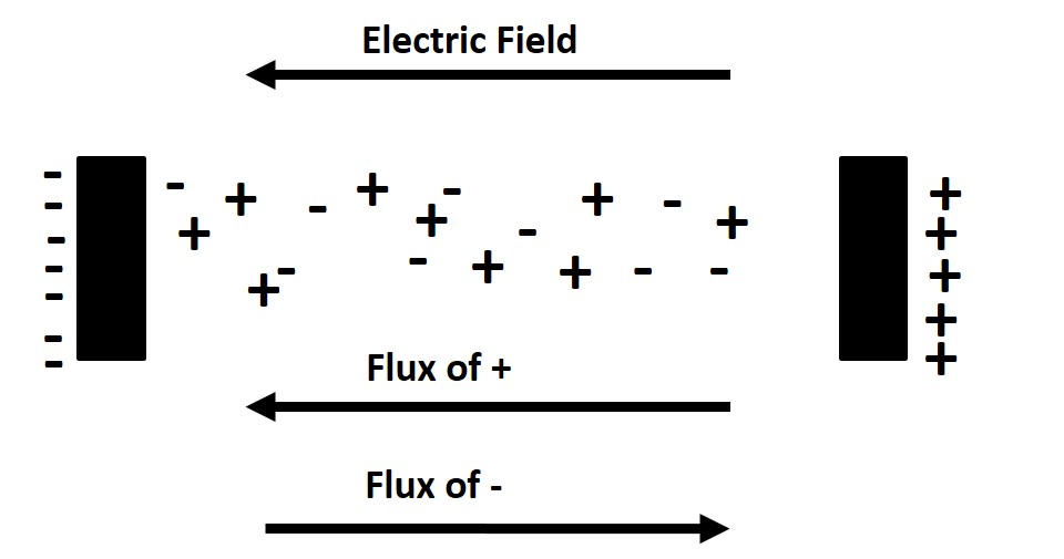
Charged Species

One example of diffusion involving charged species occurs in lithium-ion batteries, where both chemical and electric field gradients contribute to ionic flux. The total flux is the sum of these contributions. Depending on their relative magnitudes, the system may exhibit zero net flux (steady state) or even “uphill” diffusion if the electric field dominates.

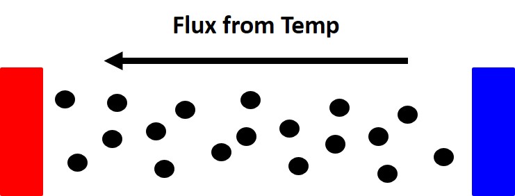
Temperature Gradients

Diffusion can also be driven by thermal gradients. Typically, atoms migrate toward regions of higher temperature because increased atomic vibration lowers activation barriers for diffusion.

Curvature Effects

Diffusion can also be driven by surface curvature. Material tends to diffuse from regions of positive curvature (convex) to regions of negative curvature (concave), smoothing the surface over time.

Stress-Driven Diffusion

Stress gradients can drive atomic motion as well. In regions of hydrostatic stress, atoms tend to diffuse from compressive regions to tensile regions. Around an edge dislocation, for example, solute atoms will diffuse toward the tensile region beneath the dislocation until a steady-state configuration is reached — this is known as a Cottrell atmosphere.

Fick’s Second Law

So far, we have considered steady-state diffusion under constant gradients, but diffusion in most materials is time-dependent. To account for this, we use Fick’s Second Law:

\[
\frac{\partial c}{\partial t} = \dot{n} - \nabla \vec{J}
\]

where \( \dot{n} \) is the rate of creation of new species (often zero) and \( \vec{J} \) is the flux. Substituting Fick’s First Law (\( \vec{J} = -D \nabla c \)) gives:

\[
\frac{\partial c}{\partial t} = D(c)\nabla^2 c + \frac{dD(c)}{dc} (\nabla c)^2
\]

This form applies when the diffusivity \( D \) depends on concentration. For most engineering cases, \( D \) is approximately constant, reducing the equation to the classical form:

\[
\frac{\partial c}{\partial t} = D \nabla^2 c
\]

This partial differential equation describes how the concentration field \( c(x,t) \) evolves with time. We can solve it for specific boundary conditions, such as a diffusion couple.

To solve this, we introduce a dimensionless variable:

\[
\eta = \frac{x}{\sqrt{4 D t}}
\]

Using this substitution, Fick’s Second Law (in one dimension) simplifies to an ordinary differential equation in \( \eta \):

\[
-2\eta \frac{\partial c}{\partial \eta} = \frac{\partial^2 c}{\partial \eta^2}
\]

The boundary conditions are:
\[
c(\eta = -\infty) = c^L, \quad c(\eta = \infty) = c^R
\]

The solution is:

\[
c(\eta) = c^L + \frac{a_1}{\sqrt{\pi}} \left( \int_0^{-\infty} e^{-\zeta^2} d\zeta + \int_0^{\eta} e^{-\zeta^2} d\zeta \right)
\]

In practice, this is equivalent to the well-known error function solution for diffusion in a semi-infinite medium.

When can we make the semi-infinite approximation?

The semi-infinite approximation applies when the diffusion length is much smaller than the specimen size:

\[
l > 10 \sqrt{D t}
\]

Engineering Approximation for Diffusion Depth

Many diffusion problems can be solved analytically using the above substitution or numerically. However, there is also a simple engineering approximation for estimating diffusion depth. The solutions to diffusion problems often have an error function (\( \mathrm{erf} \)) shape, which flattens out for \( \mathrm{erf}(x) \approx 1 \). This occurs when \( x \approx 2 \), so we can estimate the diffusion depth \( x \) as:

\[
1 = \frac{x}{2 \sqrt{D t}}
\]

This provides a quick estimate for how far atoms or species have diffused in a given time.

Arrhenius Temperature Dependence of Diffusion and Anisotropy

So far, we have discussed the concentration dependence of diffusivity \( D \), but \( D \) also depends strongly on temperature and crystal structure. The temperature dependence follows an Arrhenius relationship:

\[
D = D_0 \exp\left(\frac{-Q_a}{kT}\right)
\]

where \( D_0 \) is the pre-exponential factor and \( Q_a \) is the activation energy for diffusion.

Diffusion is also often anisotropic, especially in crystalline materials where the diffusion path length varies by direction. For example:

Cubic materials:
\[
\begin{bmatrix}
D_{11} & 0 & 0 \\
0 & D_{11} & 0 \\
0 & 0 & D_{11}
\end{bmatrix}
\]

Tetragonal or hexagonal materials:
\[
\begin{bmatrix}
D_{11} & 0 & 0 \\
0 & D_{11} & 0 \\
0 & 0 & D_{33}
\end{bmatrix}
\]

Orthorhombic materials:
\[
\begin{bmatrix}
D_{11} & 0 & 0 \\
0 & D_{22} & 0 \\
0 & 0 & D_{33}
\end{bmatrix}
\]

Monoclinic materials:
\[
\begin{bmatrix}
D_{11} & 0 & D_{13} \\
0 & D_{22} & 0 \\
D_{31} & 0 & D_{33}
\end{bmatrix}
\]

Triclinic materials:
\[
\begin{bmatrix}
D_{11} & D_{12} & D_{13} \\
D_{21} & D_{22} & D_{23} \\
D_{31} & D_{32} & D_{33}
\end{bmatrix}
\]

This shows how the crystal symmetry determines the number of independent diffusion coefficients.

Diffusion as a Random Walk

Another way to think about diffusion is as a series of discrete atomic jumps in a random walk. The diffusivity can be expressed as:

\[
D = \frac{N \Gamma \langle r^2 \rangle f}{2d}
\]

where:
- \( \langle r^2 \rangle \) is the mean squared jump distance,
- \( d \) is the dimensionality of diffusion (1D, 2D, or 3D),
- \( f \) is the correlation factor that accounts for non-random motion,
- \( N \) is the number of available neighboring sites,
- \( \Gamma \) is the atomic jump frequency.

The jump frequency is itself thermally activated and follows an Arrhenius form:

\[
\Gamma = \nu \exp\left(\frac{-G^m}{kT}\right)
\]

where \( \nu \) is the attempt frequency (on the order of atomic vibration frequencies) and \( G^m \) is the migration free energy for the atomic jump.

The correlation factor \( f \) quantifies how correlated successive atomic jumps are:
- For a perfect random walk, \( f = 1 \).
- For completely back-and-forth motion (each jump reversed by the next), \( f = 0 \).
Most diffusion processes in solids have \( f \approx 1 \).

Diffusion Mechanisms

We now apply this framework to the major diffusion mechanisms found in solids.

Vacancy Diffusion

The predominant mechanism for self-diffusion in metals (FCC, BCC, HCP) and many ionic crystals is vacancy diffusion. The atom moves by jumping into an adjacent vacant lattice site.

For an FCC crystal, the diffusivity can be expressed as:

\[
D = a^2 \nu \exp\left(\frac{S^m_v + S^f_v}{k}\right) \exp\left(\frac{-H^m_v - H^f_v}{kT}\right)
\]

where:
- \( a \) is the lattice constant,
- \( S^m_v \) and \( S^f_v \) are the migration and formation entropies of the vacancy,
- \( H^m_v \) and \( H^f_v \) are the migration and formation enthalpies,
- \( N = 12 \) for FCC (12 nearest neighbor sites),
- The jump distance is \( r = \frac{a}{\sqrt{2}} \).

Interstitial Diffusion

Interstitial diffusion occurs for small solute atoms moving through the interstitial sites of a crystal lattice of much larger atoms. This mechanism is much faster than vacancy diffusion since it does not require vacancy formation.

For example, consider the interstitial diffusion of carbon in BCC iron (ferrite). Carbon atoms occupy octahedral interstitial sites. The diffusivity is:

\[
D = \frac{a^2}{6} \nu \exp\left(\frac{S^m}{k}\right) \exp\left(\frac{-H^m}{kT}\right)
\]

where:
- \( a \) is the lattice parameter,
- \( N = 4 \) for BCC (4 neighboring octahedral sites),
- The jump distance is \( r = \frac{a}{2} \).

Other Diffusion Mechanisms

In addition to vacancy and interstitial diffusion, several other mechanisms can occur:
- Interstitialcy (kick-out) mechanism, where two atoms exchange positions cooperatively.
- Ring mechanism, common in ionic and covalent materials.
- Grain boundary diffusion and surface diffusion, which occur at higher rates due to more open atomic packing at interfaces.

Diffusion Depends on Local Environment

The diffusivity of a material also depends on its local microstructural environment — whether atoms are in the bulk lattice, near a dislocation core, along a grain boundary, or on a free surface. The relative magnitudes of diffusion coefficients are generally:

\[
D^L > D^S > D^D \approx D^B > D^{XL}
\]

where:
- \( D^L \): diffusivity in a liquid
- \( D^S \): diffusivity along a surface
- \( D^D \): diffusivity along a dislocation
- \( D^B \): diffusivity along a grain boundary
- \( D^{XL} \): bulk (crystalline lattice) diffusivity

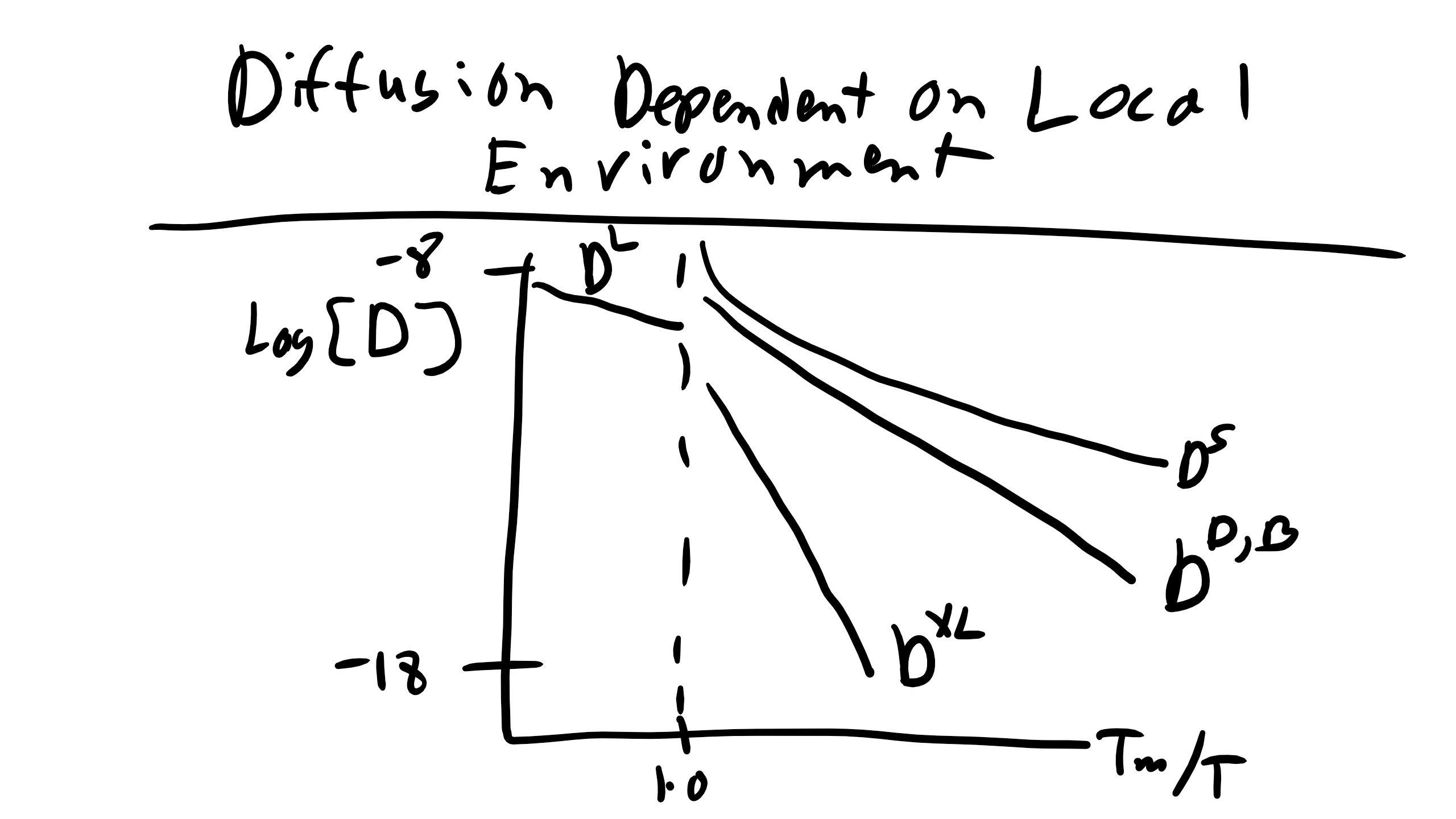
This ranking makes intuitive sense. Regions with more free volume, such as grain boundaries or surfaces, provide easier pathways for atomic migration, resulting in higher diffusivity. In contrast, atoms in a perfect crystal must rely solely on thermal vibrations to open space for diffusion, making bulk diffusion much slower.

Elastic Strain Energy of Edge Dislocation Dipoles

Let us now examine how two dislocations interact elastically. Consider two edge dislocations separated by a distance \( d \), each with Burgers vectors \( b_1 \) and \( b_2 \). The first dislocation is located at the origin. We can think of these dislocations analogously to electric dipoles — with opposite Burgers vectors, they attract; with the same Burgers vectors, they repel.

The stress field of the first dislocation produces a force on the second dislocation that can be calculated using the Peach–Koehler formalism:

\[
\overline{b}_2 = b_2 \, i, \quad \overline{t}_2 = k
\]
\[
\overline{f}_{12} = (\sigma^1 \cdot \overline{b}_2) \times \overline{t}_2 = \sigma^1_{xy} b_2 i - \sigma^1_{xx} b_2 j
\]

Focusing on motion along the x-axis, the force per unit length is:

\[
f_{12} = \sigma^1_{xy} b_2 = \frac{G b_1 b_2}{2 \pi (1 - \nu) d}
\]

This expression matches our intuition — dislocations with the same Burgers vector repel, while dislocations with opposite Burgers vectors attract and can annihilate each other.

We can also calculate the elastic strain energy associated with two dislocations by integrating the force required to move them apart from a state where they were annihilated (separation \( r_0 \)) to a separation distance \( d \):

\[
\frac{\Delta U_{edge-int}}{l} = \int_{r_0}^{d} f_{12} \, dx = \frac{G b^2}{2 \pi (1 - \nu)} \ln\left(\frac{d}{r_0}\right)
\]

This equation shows that for two dislocations of opposite Burgers vectors, the free energy decreases as they move closer together — confirming that annihilation is energetically favorable.

Dislocation Motion

Returning to dislocation motion, recall that glide occurs within the slip plane of the dislocation, while climb involves motion perpendicular to the slip plane. Climb requires the absorption or emission of vacancies or interstitials, and is therefore thermally activated.

The normal to the glide plane is given by:

\[
\overline{n} = \frac{\overline{t} \times \overline{b}}{|\overline{t} \times \overline{b}|}
\]

Note that by this definition, a pure screw dislocation does not have a unique glide plane, enabling a special mechanism known as cross-slip. Cross-slip is important for plastic deformation in metals, particularly at low temperatures, and occurs when a screw dislocation moves from one slip plane to another.

Slip Systems

Each material has a specific set of crystallographic planes and directions on which dislocations preferentially glide, known as slip systems.

For FCC materials:
\[
\text{Slip planes: } \{111\}, \quad \text{Slip directions: } \langle 110 \rangle, \quad \text{Slip system: } \{111\}\langle 110 \rangle
\]

For BCC materials:
\[
\text{Slip planes: } \{110\}, \quad \text{Slip directions: } \langle 111 \rangle, \quad \text{Slip system: } \{110\}\langle 111 \rangle
\]

These directions and planes are the most densely packed in their respective lattices. Because they minimize the energy per unit length of the dislocation, they are the most energetically favorable slip systems. In materials with high stacking fault energies (such as aluminum), dislocations tend to remain undissociated, whereas in low stacking fault energy materials (such as copper), dislocations can split into partials.

Glissile and Sessile Dislocations

Dislocations that can move easily are called glissile, while those that are immobile under applied stress are sessile. Sessile dislocations can form when dislocation reactions produce new dislocations with Burgers vectors that are not aligned with any slip system, preventing glide. Sessile dislocations play an important role in strain hardening.

Dislocation Climb

Dislocation climb requires atomic transport perpendicular to the slip plane. This process is governed by the diffusion of vacancies or interstitials to and from the dislocation core. It is therefore slow at low temperatures and becomes significant during high-temperature creep.

The motion of dislocations under applied stress can be analyzed in terms of the resolved shear stress \( \tau \) acting on the slip system. The resolved shear stress is given by:

\[
\tau = \alpha_{ij} \sigma_{ij}
\]
\[
\alpha_{ij} = \frac{1}{2} (\overline{b}_i \overline{n}_j + \overline{b}_j \overline{n}_i)
\]

Here, \( \alpha_{ij} \) is the Schmid tensor, which projects the stress tensor onto the slip system.

A critical resolved shear stress (CRSS), denoted \( \tau_{crss} \), must be reached before a dislocation can move. This is sometimes referred to as the lattice resistance. For FCC metals, \( \tau_{crss} \) is small, so dislocations glide easily. In contrast, for covalent or ionic solids (e.g., diamond or ceramics), \( \tau_{crss} \) is extremely high, and fracture often occurs before any significant plastic deformation.

Kink Motion, Climb Kinetics, and Orowan’s Equation

At low temperatures in certain materials, particularly BCC metals, dislocation motion can occur via the nucleation and migration of kinks. A kink is a step on a dislocation line within its glide plane, whereas a jog is a step that moves out of the glide plane.

For edge dislocations, jogs require mass transport (diffusion of atoms or vacancies) to move, while for screw dislocations, both steps are referred to as kinks. The motion of dislocations through kink propagation can be visualized as movement through a potential energy landscape — dislocations move through successive energy barriers, with each kink hopping from one potential minimum to the next.

Kink Motion

The formation and migration of kinks are thermally activated processes. The rate of kink motion depends on the applied stress \( \tau \), Burgers vector \( b \), and temperature \( T \). The forward and backward jump frequencies for kinks are:

\[
\Gamma_+ \approx \nu \exp\left[-\frac{(\Delta G^m_k - \frac{\tau b^3}{2})}{kT}\right]
\]
\[
\Gamma_- \approx \nu \exp\left[-\frac{(\Delta G^m_k + \frac{\tau b^3}{2})}{kT}\right]
\]

where \( \nu \) is the attempt frequency, and \( \Delta G^m_k \) is the migration free energy for kink motion. The net rate is:

\[
\Gamma = \Gamma_+ - \Gamma_- \approx 2 \nu \exp\left(-\frac{\Delta G^m_k}{kT}\right) \sinh\left(\frac{\tau b^3}{2kT}\right)
\]

At low stresses, where \( \sinh(x) \approx x \), this simplifies to:

\[
\Gamma \approx \nu \exp\left(-\frac{\Delta G^m_k}{kT}\right) \frac{\tau b^3}{2kT}
\]

The velocity of a single kink is then:

\[
v_k = b \Gamma
\]

If multiple kinks are distributed along the dislocation line, each separated by distance \( l \), the average dislocation velocity becomes:

\[
v = \frac{b^2 \nu}{l} \exp\left(-\frac{\Delta G^m_k}{kT}\right) \frac{\tau b^3}{2kT} = D_k \frac{\tau b^3}{2kT}
\]

where \( D_k \) is the kink diffusivity, which follows Arrhenius behavior.

The equilibrium concentration of kinks per unit length is given by:

\[
c_k = \frac{1}{l} = \frac{\exp\left(-\frac{\Delta G^f_k}{kT}\right)}{b}
\]

where \( \Delta G^f_k \) is the kink formation free energy. Combining these relationships gives a general mobility law for dislocations:

\[
v = D_k \exp\left(-\frac{\Delta G^f_k}{kT}\right) \frac{\tau b^2}{kT}
\]

At high stresses, dislocation velocity is governed by the nucleation and separation of kink pairs. The free energy for forming a kink pair is:

\[
\Delta G^f_{kp} = 2 \Delta G^f_k \left(1 - \frac{\tau}{\tau_{max}}\right)^2
\]

where \( \tau_{max} \) is the threshold stress beyond which no thermal activation is required to move kinks.

Dislocation Climb

Dislocation climb, unlike glide, requires diffusion of vacancies or interstitials to or from the dislocation core. The emission and trapping rates of vacancies are given by:

\[
\Gamma_{emit} = \nu \exp\left(-\frac{\Delta G^f_v}{kT}\right) \exp\left(-\frac{\Delta G^m_v - \frac{\sigma b^3}{2}}{kT}\right)
\]
\[
\Gamma_{trap} = \nu n_v \exp\left(-\frac{\Delta G^m_v + \frac{\sigma b^3}{2}}{kT}\right)
\]

where \( \sigma \) is the applied stress and \( n_v \) is the equilibrium vacancy concentration. The net rate, assuming steady-state conditions and low stress, becomes:

\[
\Gamma = \Gamma_{emit} - \Gamma_{trap} \approx \nu n_v \exp\left(-\frac{\Delta G^m_v}{kT}\right) \frac{\sigma b^3}{kT}
\]

Since climb velocity is proportional to the jump rate:

\[
v_j = b \Gamma
\]

and if there is a concentration \( c_j \) of jogs along the dislocation line, the overall dislocation climb velocity is:

\[
v = b^2 n_v c_j \nu \exp\left(-\frac{\Delta G^m_v}{kT}\right) \frac{\sigma b^3}{kT} = D_s \frac{c_j \sigma b^3}{kT}
\]

where \( D_s = D_v n_v \) is the self-diffusivity.

Orowan’s Equation for Dislocation Motion

The relationship between dislocation motion and plastic strain rate was established by Orowan, who related the strain rate to the dislocation density and velocity.

The shear strain from the passage of one dislocation is:

\[
\gamma = \frac{b}{h} = \frac{bA}{V}
\]

For incremental dislocation motion \( dx \):

\[
d\gamma = b \frac{dA}{V} = \frac{b l dx}{V}
\]

For \( n \) dislocations:

\[
d\gamma = \frac{n b l dx}{V}
\]

Since dislocation density \( \rho = \frac{n l}{V} \), we can express this as:

\[
d\gamma = b \rho dx
\]

and differentiating with respect to time gives:

\[
\dot{\gamma} = b \rho v
\]

This is the Orowan equation, a fundamental relationship linking the macroscopic plastic strain rate \( \dot{\gamma} \) to microscopic dislocation properties. It tells us that plastic deformation rate increases with dislocation density, Burgers vector magnitude, and dislocation velocity.

Dislocation Reactions, Sources, and Sessile Dislocations

We have covered the forces on dislocations, their stress fields, and mobility. Now, we turn to interactions between dislocations that can either increase or decrease the yield strength of a material. These interactions are collectively referred to as dislocation reactions.

When two dislocations meet, they can react with one another, and these reactions can occur spontaneously if the total energy of the system decreases. The Burgers vector of the resulting dislocation is the vector sum of the Burgers vectors of the reactants.

According to Frank’s Rule, the energy per unit length of a dislocation is proportional to the square of its Burgers vector. Therefore, a dislocation reaction is energetically favorable (spontaneous) if:

\[
b_{product}^2 < b_1^2 + b_2^2
\]

A simple example of this is the annihilation of two dislocations with equal and opposite Burgers vectors, producing a perfect crystal with \( b_{product} = 0 \).

Generating New Dislocations

There are several mechanisms by which new dislocations can form in a material:

1. Generation from Dislocation Sources
2. Heterogeneous Nucleation
3. Homogeneous Nucleation

Generation of New Dislocations from Dislocation Sources

One of the most important and efficient ways to generate new dislocations is through the Frank–Read (FR) source. Imagine a dislocation segment pinned at both ends. When a shear stress is applied, the dislocation bows out in the direction of the applied force. The opposing force is the line tension due to the dislocation’s curvature.

The curvature \( \kappa \) of the bowed-out dislocation is:

\[
\kappa = \frac{1}{r}
\]

Initially, when the dislocation is straight, the curvature is zero because \( r \to \infty \). As the dislocation bows out, the curvature increases, reaching a maximum when \( r = \frac{l}{2} \). The critical resolved shear stress required to reach this condition is found by equating the applied force per unit length (\( \tau_c b \)) to the maximum line tension (\( \frac{G b^2}{4\pi R} \)):

\[
\tau_c b = \frac{G b^2}{2 \pi l}
\]
\[
\tau_c = \frac{G b}{2 \pi l}
\]

Beyond this point, further bowing reduces the curvature, and the dislocation eventually loops back on itself. The two opposing segments of the dislocation annihilate where they meet, leaving behind a closed dislocation loop and reestablishing the original pinned segment — now ready to repeat the process. This mechanism can produce a large number of dislocation loops from a single source under constant applied stress.

There also exists a single-ended version of this source, where the dislocation is pinned at only one end and spirals outward, known as a spiral Frank–Read source. Another related mechanism is the Bardeen–Herring (BH) source, which operates through dislocation climb rather than glide.

Heterogeneous Dislocation Nucleation

Dislocations can also nucleate heterogeneously at existing defects such as grain boundaries, free surfaces, or other dislocations. This type of nucleation requires less stress than homogeneous nucleation because the presence of a defect reduces the energy barrier for dislocation formation. However, since the nucleus is on the atomic scale, linear elasticity theory cannot describe it accurately, and atomistic modeling is typically required.

Homogeneous Dislocation Nucleation

Homogeneous nucleation refers to dislocation formation within a perfect crystal, without the aid of preexisting defects. It requires extremely high stresses, close to the theoretical shear strength of the material (\( \approx G / 10 \)). Homogeneous nucleation typically involves the formation of dislocation loops, as dislocations cannot start or end inside a perfect lattice. This mechanism is rare and generally only occurs under very high applied stresses, such as during shock loading or intense deformation.

Formation of Sessile Dislocations

Certain dislocation reactions produce dislocations that are sessile — meaning they cannot move by glide. Sessile dislocations play a key role in strain hardening because they act as obstacles to dislocation motion, increasing the yield strength.

A well-known example occurs in FCC metals through the Lomer–Cottrell reaction. Two glissile dislocations on intersecting {111} planes react to form a sessile dislocation along the line of intersection of the two planes.

An example reaction is:

\[
\frac{a}{2}[\overline{1}10] + \frac{a}{2}[101] \rightarrow \frac{a}{2}[011]
\]

The magnitudes of the Burgers vectors are \( b_{reactants}^2 = a^2 \) and \( b_{product}^2 = \frac{a^2}{2} \), so the reaction is energetically favorable. The resulting dislocation lies on the (100) plane and has the slip system (100)[0\overline{1}1], which is not a normal glide plane, making the dislocation sessile.

Because sessile dislocations require energy input to dissociate and move, they act as pinning points, preventing the motion of other dislocations. Even short sessile segments can effectively block gliding dislocations, leading to increased hardening. In low stacking fault energy (SFE) FCC metals, dislocations may dissociate into partials (Shockley partials), leading to similar blocking effects.

Types of Plastic Behavior and Yield Criteria

We have now built a foundation for understanding plasticity from the atomistic perspective, so we can step back and take a more macroscopic view of how materials yield. There are several types of plastic behavior that materials can exhibit.

Rigid/Perfectly Plastic Behavior

In a rigid or perfectly plastic material, the material behaves as if it were completely rigid (infinite Young’s modulus) up to the yield point. Once yielding occurs, the material deforms plastically at a constant stress. There is no strain hardening or softening.

Elastic/Perfectly Plastic Behavior

A more realistic model assumes that the material exhibits elastic behavior up to the yield point, after which plastic deformation occurs at a constant yield stress.

Elastic/Strain Hardening Behavior

Many ductile materials exhibit strain hardening, where the stress required to continue plastic deformation increases with strain. After yielding, the true stress–strain relationship can be expressed as:

\[
\sigma = \sigma_y + k \epsilon^n
\]

where \( n \) is the strain-hardening exponent, typically ranging from 0.1 to 0.5 for metals.

Elastic/Strain Softening Behavior

Some materials, such as certain polymers and metallic glasses, exhibit strain softening after yielding — the stress decreases with continued strain.

These idealized material behaviors allow us to model and predict how materials respond once they enter the plastic regime. Next, we turn to the criteria that define when yielding begins.

Yielding Criteria

To predict yielding under complex, multiaxial loading states, several yield criteria have been developed. Before introducing them, we make the following assumptions:

1. Plastic flow occurs at constant volume.
2. Modest hydrostatic pressure does not cause yielding (\( p < E/100 \)).
3. The material is perfectly plastic.
4. The material is isotropic.

Under these assumptions, we can apply the Rankine, Tresca, and von Mises yield criteria.

Rankine Criterion

The Rankine or maximum normal stress criterion states that a material yields when the maximum principal stress \( \sigma_1 \) reaches the yield stress observed in uniaxial tension:

\[
\sigma_1 \geq \sigma_y
\]

This criterion does not account for shear stresses and therefore cannot accurately describe yielding in most ductile materials.

Tresca Criterion

The Tresca or maximum shear stress criterion assumes that yielding occurs when the maximum shear stress reaches the critical value measured under uniaxial loading. The maximum shear stress is given by:

\[
\tau_{max} = \frac{\sigma_1 - \sigma_3}{2}
\]

and yielding occurs when:

\[
\sigma_1 - \sigma_3 \geq \sigma_y
\]

This model improves upon Rankine’s by incorporating shear stresses, but experimental evidence during World War I and II showed it to be a poor predictor for certain metals, such as those used in submarine hulls.

Von Mises Criterion

The von Mises or maximum shear deformation energy criterion states that yielding occurs when the distortion energy reaches the same value as at the onset of yielding in a uniaxial tension test. The effective stress is defined as:

\[
\sigma_{eff} = \sqrt{\frac{1}{2}[(\sigma_{11}-\sigma_{22})^2 + (\sigma_{22}-\sigma_{33})^2 + (\sigma_{33}-\sigma_{11})^2 + 6(\sigma_{23}^2 + \sigma_{31}^2 + \sigma_{12}^2)]}
\]

Yielding occurs when:

\[
\sigma_{eff} \geq \sigma_y
\]

In terms of the principal stresses:

\[
\sigma_{eff} = \sqrt{\frac{1}{2}[(\sigma_1 - \sigma_2)^2 + (\sigma_2 - \sigma_3)^2 + (\sigma_3 - \sigma_1)^2]} \geq \sigma_y
\]

When these yield surfaces are plotted in principal stress space, the von Mises yield locus forms a cylinder, while the Tresca criterion forms a hexagon. The von Mises surface provides a smoother, more accurate description of yielding in ductile materials and is widely used in modern engineering design.

Polymer Yielding: Shear Banding and Crazing

Shear Banding

Shear bands are localized zones of intense plastic deformation and chain alignment, typically thousands of nanometers wide. They nucleate at stresses near \( G / 10 \) and continue to grow as stress increases. Shear bands form at approximately 45° to the applied tensile axis (the planes of maximum shear stress) and are highly temperature-dependent.

Interestingly, the yield stress in compression is generally higher than in tension. This asymmetry is especially pronounced in polymers, where tensile loading tends to open free volume and promote chain alignment, making yielding easier.

Crazing

Crazes are another form of localized plastic deformation, distinct from cracks. They consist of microvoids and fibrils that span the deformed region. Crazes form perpendicular to the applied tensile axis, with fibrils aligned parallel to the loading direction. They do not form under compressive stress.

Shear banding and crazing can be thought of as polymer-specific manifestations of yielding. In modeling, the von Mises criterion can be modified to account for shear banding, and the Tresca criterion can be applied to describe crazing.

Strengthening Mechanisms

We have previously seen how dislocation motion controls plastic deformation, and we now know that yield stress depends on the ease with which dislocations move. One of the most powerful aspects of materials science is that we can intentionally modify a material’s structure to change how dislocations move — and thereby tune the yield strength. This ability to tailor mechanical properties based on structure–processing relationships is a central theme of the materials tetrahedron.

The general principle is simple: the yield stress increases when it becomes harder for dislocations to move or propagate. Obstacles to dislocation motion raise the stress required for yielding. There are four primary strengthening mechanisms:

1. Work Hardening
2. Solute Strengthening
3. Grain Size Strengthening
4. Precipitate/Particle Strengthening

Work Hardening (Lattice Resistance)

Dislocation density is a measure of the total length of dislocations per unit volume or, equivalently, the number of dislocations per area of a slip plane. It is given by:

\[
\rho = \frac{N}{A}
\]

where \( N \) is the number of dislocations in area \( A \). A heavily cold-worked material typically has a dislocation density on the order of \( 10^{14} \, \text{m}^{-2} \), while a well-annealed material may have only \( 10^7 \, \text{m}^{-2} \).

The average distance between dislocations can be approximated as:

\[
\rho = \frac{1}{l^2}
\]

where \( l \) is the spacing between dislocations. The increase in yield stress due to dislocation interactions can then be written as:

\[
\Delta \sigma_y = \alpha G b \sqrt{\rho}
\]

where \( G \) is the shear modulus, \( b \) is the Burgers vector, and \( \alpha \) is a material constant (typically near 1).

Plastic deformation increases dislocation density as new dislocations are generated. As these dislocations interact and tangle, they impede each other’s motion, making further deformation more difficult — this is work hardening. Rolling, drawing, or hammering metals are practical examples of inducing work hardening.

Alternatively, annealing a material (heating to elevated temperature) allows dislocations to climb and annihilate at free surfaces, reducing dislocation density and restoring ductility. During annealing, the grain size increases roughly as \( d \sim t^{1/2} \), where \( t \) is time.

When solute atoms are added to a host metal, they can distort the local lattice because of differences in atomic size or modulus. These localized stress fields interact with dislocations and impede their motion.

The increase in yield strength due to solute atoms can be expressed as:

\[
\Delta \sigma_y = G b \sqrt{c_{sol}} \, \epsilon_{sol}^{3/2}
\]

where \( c_{sol} \) is the solute concentration and \( \epsilon_{sol} \) is the lattice strain caused by size mismatch between solute and solvent atoms. The modulus mismatch between solute and solvent atoms can also contribute to strengthening.

The strengthening effect increases with solute concentration up to the solubility limit. This mechanism explains why solid-solution alloys (e.g., brass, bronze, stainless steel) are stronger than their pure metal components.

Grain Size Strengthening

Another effective way to increase strength is by reducing grain size. Grain boundaries act as barriers to dislocation motion, since dislocations cannot easily transmit across boundaries with different crystallographic orientations.

The Hall–Petch relationship describes this effect:

\[
\Delta \sigma_y = \frac{\kappa}{d_g}
\]

where \( \kappa \) is a material constant and \( d_g \) is the grain diameter. Smaller grains provide more grain boundaries, leading to higher yield strength.

However, this strengthening effect does not continue indefinitely. When the grain size becomes very small (below about 10 nm), dislocations cannot form or pile up inside the grain, and other deformation mechanisms such as grain boundary sliding dominate. As a result, the yield strength eventually decreases — a phenomenon known as the inverse Hall–Petch effect.

Precipitate/Particle Strengthening

In precipitation-hardened or particle-strengthened materials, dislocations encounter second-phase particles that serve as obstacles to motion. Depending on particle size and spacing, dislocations can either cut through the particles or bow around them.

If the dislocation cuts through particles, the strengthening effect is given by:

\[
\Delta \sigma_y = \frac{\gamma_{p-m} \pi r_p}{b l} = \kappa^3 \sqrt{r_p f_p}
\]

where:
- \( \gamma_{p-m} \) is the interfacial energy between the particle and the matrix,
- \( r_p \) is the particle radius,
- \( l \) is the average spacing between particles,
- \( f_p \) is the particle volume fraction, and
- \( \kappa \) is a constant related to particle geometry.

When dislocations bypass particles through bowing (the Orowan mechanism), the strengthening effect is:

\[
\Delta \sigma_y = \frac{G b}{l - 2 r_p}
\]

where \( G \) is the shear modulus, \( b \) is the Burgers vector, \( l \) is the particle spacing, and \( r_p \) is the particle radius.

For small particles, cutting is energetically more favorable because the interfacial energy penalty is low. For large particles, bowing becomes more favorable because cutting would require the creation of a large new interfacial area. Increasing the volume fraction of particles reduces the critical radius for transition between cutting and bowing, since more interfaces are created during cutting.

These four strengthening mechanisms — work hardening, solute strengthening, grain size strengthening, and precipitate strengthening — are often combined in engineering materials to achieve the desired balance of strength, ductility, and toughness.