Chapter 8: Beam Bending, Buckling, and Torsion

Elastic Loading Topics: Bending, Buckling, and Torsion

Before we move into plasticity, we have three elastic loading topics to discuss, and these are still very important and relevant loading states and phenomena: bending, buckling, and torsion respectively.

You have probably already encountered beam bending in other courses and perhaps buckling, but we again are going to take a slightly different approach—specifically approaching this from the materials perspective.

We can define a beam as anything that can carry transverse loads. This can range from typical civil engineering structural applications (bridges, trusses, pool diving boards, etc.) to more exotic applications like Atomic Force Microscopy (AFM), which utilizes a cantilever beam, or thin-film substrates that have thermal mismatch resulting in bending. Other examples include cellular solids like foams, honeycomb structures, tissues, and even sporting equipment like ski poles.

When dealing with beam bending problems, we must consider several things before we start to approach the problem. Specifically, we must consider:

- Support Reactions
- Internal Forces
- Internal Moments
- Internal Stresses
- Deflections
- Support Type: roller, pin, or fixed end

Additionally, different supports will have different reaction forces and moments. For example:

- Roller: Reaction force in the y-direction
- Pin: Reaction force in the x and y directions
- Simple Frictionless Surface: Reaction force in the y-direction
- Fixed Support: Reaction forces in x, y, and a reaction moment

Soon we will be working with free body diagrams as well as shear force and moment distributions within structures. Why do we want to do this? We need to find the locations of maximum shear forces and bending moments because material failure will often occur at regions of maximum shear forces (denoted as \( V \)) and bending moments (\( M \)). These shear forces and bending moments can vary along the length of the beam. Moreover, shear stress depends on the shear forces, whereas normal stresses depend on the bending moment. Finally, the amount of deflection will also depend on the bending moment.

Let's start off with some background on how we will work with beams and support reaction diagrams. This should have been covered in other courses, but let's give ourselves a quick reminder.

Sign Convention and Coordinate System Reminder

Before we get started, let’s do one more reminder of our coordinate system and what we will determine as positive and negative forces, shears, and moments.

- Tension will be defined as positive.
- Compression as negative.
- Shear is positive if the force is acting on a face with a normal in the positive direction and also has a force pointed in the positive direction.

For forces, any force which points in the positive direction relative to our coordinate system will be defined as positive. Counterclockwise (CCW) moments are positive, and clockwise (CW) moments are negative.

For beams:
- A positive internal shear force \( V \) acts downward on the right-hand face of a beam or upward on the left-hand face of a beam.
- A positive internal bending moment \( M \) acts CCW on the right-hand face of the beam and CW on the left-hand face of a beam.

You can also consider a bending moment as positive if tension is on the bottom of the beam and negative if tension is at the top.

The key point to this entire discussion is that before you approach any mechanics problem, if there is not a coordinate system defined, you must define one before you start anything. Keep this in mind—it will be very important that you double-check this as you approach problems.

Support Reactions in Beams

Let's first consider a fixed-end supported cantilever beam of length \( l \) with a load \( P \) applied at the end. At the fixed end we will have one reaction force \( F_y \) and a reaction moment \( M_0 \).

For virtually all of our beam bending problems we will start as follows to develop our problem-solving framework:

1. Coordinate System
2. Free Body Diagram
3. Equilibrium Expressions
4. Solve for Unknowns

As you can see below we have defined our coordinate system and we have drawn our free body diagram. Now we can apply our equilibrium conditions, remembering that we have:

\[
\Sigma F = 0
\]
\[
\Sigma M = 0
\]

Let's start as we always will and draw the Free Body Diagram (FBD).

So for this scenario we will have the following equilibrium conditions:

\[
\Sigma F_y = 0 = -P + F_{y}
\]
\[
\Sigma M_{0} = 0 = M_{0} - Pl
\]

Hopefully that has jogged some memories! Let's do another one of these types of reminder problems with a distributed load on a beam that has a roller support at A and a pin at B. You can see the distributed load as well as a directly applied load. Let's do our static equilibrium problem:

\[
\Sigma F_y = 0 = F_A - P - 1 + F_B
\]
\[
\Sigma M_A = 0 = F_B (6\,m) - 1\frac{kN}{m}(6\,m)(3\,m) - 12\frac{kN}{m}(4\,m)
\]

Fixed-End Support Cantilever Beam with Point Load Applied

Now that we have some of the fundamentals down and we remember them, let's actually go ahead and start with our first shear force diagram \( V(x) \) and our bending moment diagram \( M(x) \) for an end-loaded cantilever beam that has a fixed-end support.

Let's start as always with our free body diagram (FBD), but we also have some additional steps to our algorithm:

1. Coordinate System
2. Free Body Diagram
3. Equilibrium Expressions
4. Solve for Unknowns
5. Cut beam starting at \( x = 0 \) right before the first applied load
6. Write equilibrium equations again and then solve for the internal shear moment and bending moment of the beam

We have to make a cut along some point \( x \) from the fixed-end support of our beam and draw a free body diagram to determine our static equilibrium equations. When we cut our beam, it is often easiest to start with the shear forces before we get into moments.

We know that for a fixed-support beam we will have a reaction force that opposes the load applied at the end, and this will be positive in this system. Additionally, once we make our cut, the internal shear will be negative relative to this applied force.

In terms of moments, we know that we will have a positive moment at our fixed support, and at the end of our cut component/free body diagram we will have a negative internal moment. With this conceptual understanding we can work on our equilibrium expressions and obtain:

\[
\Sigma F_y = 0 = P - V
\]
\[
\Sigma M_x = 0 = Pl - Px - M
\]

and thus we get the equations for our internal shear force and bending moment as a function of \( x \):

\[
V(x) = P
\]
\[
M(x) = P(l - x)
\]

We can see in our diagram that the shear force is independent of distance along the beam, but the maximum bending moment occurs at the fixed end—as we might have intuitively predicted before this problem. Note that due to our convention, we will state that we have a negative bending moment due to the fact that there is tension at the top of our beam.

Four-Point Bending

Let's do another problem for a very common mechanical test: four-point bending.

Consider the four-point bending scenario below where two loads are applied on a roller and pin support.

As always, let's start with our FBD.

Here we are going to have to take two cuts in order to solve this problem. If we look at our first cut near position 1, we will have the following equilibrium conditions:

\[
\Sigma F_y = 0 = P - V
\]
\[
\Sigma M_{x1} = 0 = M - Px
\]

and thus we get the equations for our internal shear force and bending moment as a function of \( x \):

\[
V(x) = P
\]
\[
M(x) = Px
\]

Note that we do not have a reaction moment at either support. Also, we should recognize the symmetry in this problem, so we only have to make two cuts because everything else is exactly the same.

For our second cut we can see:

\[
\Sigma F_y = 0 = -V + P - P
\]
\[
\Sigma M_{x2} = 0 = M - Px - P\left(x - \frac{l}{4}\right)
\]

and thus we get the equations for our internal shear force and bending moment as a function of \( x \):

\[
V(x) = 0
\]
\[
M(x) = \frac{Pl}{4}
\]

Distributed Load on a Beam with Roller and Pin Supports at the Ends

Let’s analyze a simply supported beam (roller at A, pin at B) under a uniformly distributed load (UDL) of intensity \( q \) over the full span \( l \).

We can replace the distributed load by an equivalent concentrated load:

\[
dF = q\,dx \quad \Rightarrow \quad F = \int_0^l q\,dx = ql
\]

The line of action of the equivalent force passes through the centroid of the loaded region:

\[
x_F = \frac{\int_0^l x\,dF}{F} = \frac{\int_0^l x\,q\,dx}{ql} = \frac{ql^2/2}{ql} = \frac{l}{2}
\]

Support Reactions

By symmetry (or equilibrium equations):

\[
\Sigma F_y = 0 = F_A + F_B - ql
\]
\[
\Sigma M_A = 0 = F_B l - ql \frac{l}{2}
\]
\[
F_A = F_B = \frac{ql}{2}
\]

Shear and Moment Equations

Now make a cut at a distance \( x \) from A ( \( 0 \le x \le l \) ) and write the equilibrium equations for the left segment.

Shear equilibrium:

\[
\Sigma F_y = 0 = -V - qx + F_A
\]
\[
V(x) = -qx + \frac{ql}{2} = q\left(\frac{l}{2} - x\right)
\]

Moment equilibrium about the cut:

\[
\Sigma M_x = 0 = M - F_A x + (qx)\frac{x}{2}
\]
\[
M(x) = F_A x - \frac{q x^2}{2} = \frac{qlx}{2} - \frac{q x^2}{2}
\]

Differential Relationships (useful checks)

\[
q(x) = -\frac{dV}{dx}, \quad V(x) = \frac{dM}{dx}
\]

Check with our equations:

\[
V(x) = q\left(\frac{l}{2} - x\right) \Rightarrow \frac{dV}{dx} = -q \Rightarrow q = -\frac{dV}{dx}
\]
\[
M(x) = \frac{qlx}{2} - \frac{q x^2}{2} \Rightarrow \frac{dM}{dx} = \frac{ql}{2} - qx = V(x)
\]

Everything checks perfectly.

Key Takeaways
- Under a uniform load \( q \), the shear force \( V(x) \) varies linearly and the bending moment \( M(x) \) varies quadratically.
- Maximum shear occurs at the supports, and maximum bending moment occurs at midspan.
- The identities \( q = -\frac{dV}{dx} \) and \( V = \frac{dM}{dx} \) are excellent tools for checking your diagrams.

Stresses in Beams

Beam Bending Assumptions

So far we have demonstrated that when we apply a load on a beam, internal shear and bending moments are created. This gives rise to both shear and normal stresses, and typically as we will show, the normal stresses are much greater than shear stresses, in particular when the length-to-height ratio of the beam is large, i.e. \( \frac{l}{h} > 10 \). Again, our entire purpose of learning about this topic is to avoid material failure, so we will focus on regions of maximum stress.

Now in doing so we will make several critical assumptions:

- The beam is straight.
- The material is linear elastic, isotropic, and cubic.
- The cross-section is symmetric.
- The beam is stable (no lateral buckling).

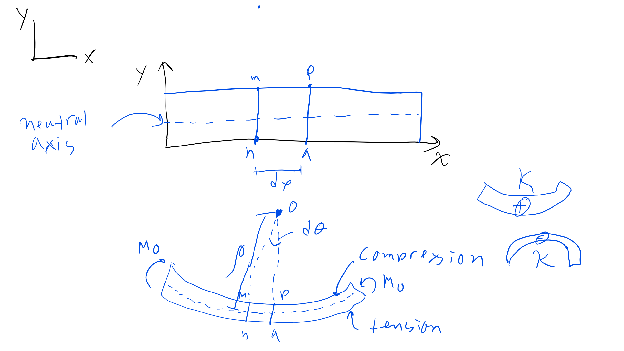
Thus, as the schematic below indicates, we will typically be dealing with scenarios as we have done previously, where one face is in tension and the other is in compression. There is also a plane along the longitudinal axis called the neutral axis that experiences no stress.

We must also distinguish between pure bending, which exhibits a constant bending moment, and non-uniform bending, where the bending moment is not constant.

Typically when we bend a beam such that it experiences positive bending near the top, the beam will be in compression, and as we move toward the bottom of the beam (height-wise), we transition from compression to no stress at the neutral axis, and then tension at the bottom of the beam.

If the material is brittle, failure will occur via crack propagation in the tensile region, whereas if a material is weak under compression, failure will occur via buckling at the top surface. We have a good idea conceptually of what is going on, but now we need to develop an expression that will tell us how this stress is distributed in a beam.

We will derive this relationship in three steps:

1. Geometric Statement
2. Constitutive Equation
3. Equilibrium Conditions

Geometric Statement

Looking at the schematic of the beam, we can clearly see that sections \( \overline{mn} \) and \( \overline{pq} \) will rotate with respect to one another, and if we extrapolate these lines, they intersect at a point \( O \), the center of curvature. The distance from \( O \) to the neutral axis is given by the radius of curvature \( \rho \). We assume that the distance between \( \overline{mn} \) and \( \overline{pq} \) at the neutral axis is constant \( dx \), so we can develop the following relationship for curvature:

\[
\kappa = \frac{1}{\rho} = \frac{d\theta}{dx}
\]

If we have pure bending, \( \rho \) is constant; it will not be if we have non-uniform bending. Additionally, curvature has the same sense of positive and negative as the bending moment.

Constitutive Equation

We can now obtain the normal strain in the x-direction, because we know that longitudinal planes other than the neutral axis will change length and produce strain in this direction. Consider a segment \( \overline{ef} \) at a distance \( y \) from the neutral axis.

We find that:

\[
l_o = dx = \rho d\theta
\]
\[
l_i = (\rho - y)d\theta
\]
\[
\epsilon_{xx} = \frac{l_i - l_o}{l_o} = -\frac{y}{\rho} = -y\kappa
\]

We see that when \( y \to 0 \), the strain also goes to 0 at the neutral axis. When \( y \) is positive, we have negative (compressive) strain at the top of the beam and vice versa for the bottom—all matching intuition.

Assuming linear elasticity, we can use Hooke’s Law:

\[
\sigma_{xx} = E \epsilon_{xx} = -E y \kappa
\]

The stress varies linearly from the neutral axis. Because we are dealing with uniaxial bending stress in the x-direction, we also have the following strain components:

\[
\epsilon_{xx} = -y \kappa
\]
\[
\epsilon_{yy} = \nu y \kappa
\]
\[
\epsilon_{zz} = \nu y \kappa
\]

We can also define transverse curvature (anelastic curvature):

\[
\kappa_{xx} = -\frac{\epsilon_{xx}}{y}, \quad
\kappa_{yy} = -\frac{\epsilon_{yy}}{y}, \quad
\kappa_{zz} = -\frac{\epsilon_{zz}}{y}
\]

Equilibrium Conditions

Now we apply equilibrium conditions to relate stress to the bending moment. For a differential element \( dA \):

\[
\Sigma F_x = 0 = \int_A \sigma_{xx} dA = \int_A -yE\kappa dA
\]

Since neither \( E \) nor \( \kappa \) is zero, the only way for the total force to be zero is if:

\[
\int_A y dA = 0
\]

which means the centroid \( \overline{y} = 0 \). Thus, the neutral axis passes through the centroid of the cross-section.

Next, consider the bending moment at the centroid (origin). The total moment must balance the distributed stress:

\[
\Sigma M_o = 0 = -M - \int_A \sigma_{xx} y dA
\]
\[
M = - \int_A \sigma_{xx} y dA = E \kappa \int_A y^2 dA
\]

Define the second moment of area (moment of inertia):

\[
I = \int_A y^2 dA
\]

For common cross-sections:

- Rectangular beam: \( I_z = \frac{b h^3}{12} \)
- Circular beam: \( J = \int_A r^2 dA = \int_A (z^2 + y^2)dA = 2I_z = \frac{\pi r^4}{4} \)

Now we can write the bending moment as:

\[
M = E \kappa I
\]

and the bending stress as:

\[
\sigma_{xx} = -E \kappa y = -\frac{M y}{I}
\]

When the bending moment is positive and \( y \) is positive, we have compression at the top and tension at the bottom.

We can also derive the strain energy due to bending per unit volume \( U_b \):

\[
U_b = \int_V U_{ESE} dV = \int_l \int_A \frac{\sigma_{xx}^2}{2E} dA dl
= \int_l \frac{M^2}{2 E I} dl
\]

A very useful relationship in beam design, as it links strain energy to the moment and stiffness.

Beam Deflection

Thus far we have been focused almost exclusively on the forces, bending, and the stresses that develop in a beam when a load is applied. However, it is often extremely important to know how far a beam will deflect from the neutral axis. This is critical because certain materials or applications will have limitations on the amount of deflection that can occur. Additionally, we can also easily measure the amount of deflection and then back out the load or material properties as well.

Let’s take a look at a beam bending scenario below where we have some given amount of deflection \( v \) and an angle \( \theta \) that describes the angle between the x-axis and the tangent to the deflection curve. The question becomes: what is the deflection at \( m_2 \)?

We know that:

\[
\rho d\theta = ds
\]
\[
\kappa = \frac{1}{\rho} = \frac{d\theta}{ds}
\]

Using the small angle approximation:

\[
\cos \theta = \frac{dx}{ds} \approx 1
\]

therefore \( ds \approx dx \), so we can obtain another expression for curvature:

\[
\kappa = \frac{d\theta}{ds} = \frac{d\theta}{dx} = \frac{d^2v}{dx^2}
\]

and we can also write:

\[
\frac{d\theta}{dx} = \frac{d^2 v}{dx^2} = \frac{M}{EI}
\]

This is a very useful relationship because we can integrate \( M(x) \) twice to get the deflection \( v(x) \), and obtain constants of integration by establishing boundary conditions. Additionally, this term \( EI \) is referred to as the flexural rigidity, a key quantity for deflection.

The Euler–Bernoulli Equation

We can develop a more general equation for beam bending using the Euler–Bernoulli beam equation, which rearranges the above in terms of a general distributed load \( q(x) \):

\[
\frac{d^2}{dx^2}\left(EI \frac{d^2v}{dx^2}\right) = q(x)
\]

If the flexural rigidity \( EI \) is constant, we can simplify this to:

\[
EI \frac{d^4v}{dx^4} = q(x)
\]

We can also relate this equation to bending moments and shear forces:

\[
M = -EI \frac{d^2v}{dx^2}
\]
\[
V = -\frac{d}{dx}\left(EI \frac{d^2v}{dx^2}\right)
\]

Thus, we have a 4th-order differential equation that we must solve to find the equation for beam deflection, requiring four boundary conditions.

Boundary Conditions for Beam Bending

It is critical to observe that the bending moment is related to the second derivative of the deflection, and the shear force is related to the third derivative of displacement. This will be important as we determine boundary conditions.

Common boundary conditions:
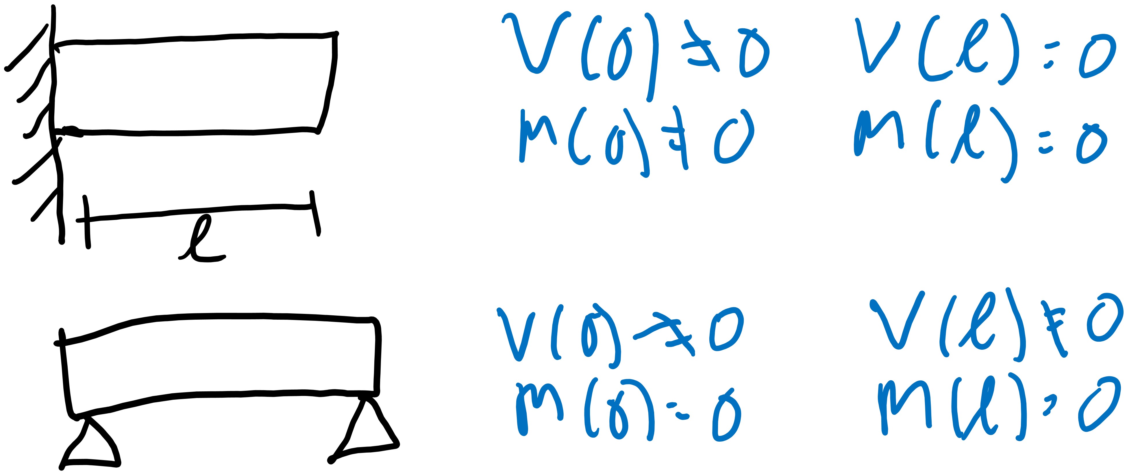
- For a cantilever beam, at the fixed support there can be no deflection or slope:
\[
v(0) = 0, \quad v'(0) = 0
\]
At the free end (no external moment or shear):
\[
v''(l) = 0, \quad EI v'''(l) = P
\]
- For a simply supported beam, there is no deflection at the supports (\( v = 0 \)), but the slope \( v' \) is not necessarily zero; the bending moment is zero at the supports.

Deflection Examples: Cantilever, 3-Point, and Distributed Load

Deflection for Simple End-Loaded Cantilever Beam with Fixed Support

Let’s look at the simple cantilever beam problem below. We can identify several boundary conditions.

For a cantilever beam:
- At the wall (fixed end), the beam will not deflect, and the slope of deflection should also be zero.
\[
v(0) = 0, \quad v'(0) = 0
\]
- At the free end, there will be no bending or shear moment:
\[
v''(l) = 0, \quad EI v'''(l) = P
\]

The differential equation for the deflection curve is given by the Euler–Bernoulli relation:
\[
EI \frac{d^4 v}{dx^4} = 0
\]

Solving this equation with the given boundary conditions, we can find the expression for deflection using symbolic or numerical tools such as Mathematica.

Three-Point Bending Test

Now let’s consider the very common three-point bending test.

For this beam, the load \( P \) is applied at the midpoint of a simply supported beam of length \( l \).
The governing equation is:
\[
EI \frac{d^4 v}{dx^4} = 0
\]
and the boundary conditions are:
\[
v(0) = 0, \quad v(l) = 0, \quad M(0) = M(l) = 0
\]
Solving this system yields the deflection profile, with the maximum deflection at midspan:
\[
v_{max} = \frac{P l^3}{48 EI}
\]

Distributed Load Example

We can also analyze a simply supported beam with a uniform distributed load \( q \).

The governing differential equation is now:
\[
EI \frac{d^4 v}{dx^4} = q
\]

Solving for \( v(x) \) using the appropriate boundary conditions for a simply supported beam:
\[
v(0) = 0, \quad v(l) = 0, \quad M(0) = M(l) = 0
\]
yields the maximum deflection:
\[
v_{max} = \frac{5 q l^4}{384 EI}
\]

All of these examples demonstrate how beam deflection can be predicted analytically by solving differential equations under the correct boundary conditions.

Buckling

When a material is placed under compression, the material will not typically fail via crack propagation, as compressive stress does not assist in crack propagation (typically). Instead, many materials under pure compressive stress will fail via buckling.

We will examine a particularly important and ubiquitous case: column buckling. A column is defined as a long, slender member that is loaded in compression, and buckling is an instability phenomenon. When we mention stability, we are referring to whether the system will return to its initial state when perturbed.

- A stable system will return to its initial state.
- An unstable system will not return to its initial state.

You have likely seen this illustrated in a physics course where a ball rolling down a hill is unstable, but one at the bottom of a well is stable. There are also neutral and metastable systems, but more on that in other courses.

Now, you may imagine that a longer column will buckle at lower applied loads, and if we increase the cross-sectional area, it will increase the applied load required for buckling. Buckling is associated with a change in shape—bending occurs. Let’s develop a framework to describe buckling.

Ideal Column with Pinned Ends

Let’s start with an ideal column with pinned ends. We will assume:
- The beam is straight.
- The material is linear elastic.
- The load is perfectly aligned with the column axis.

As the column is loaded, buckling will proceed through several stages:
1. Elastic shortening — the column is stable and compresses linearly.
2. At a critical load, instability begins — the column bends laterally.

What is this critical load, and how does it relate to the flexural modulus, beam length, and geometry?

We start by defining our coordinate system and drawing a free body diagram. The deflection at the top of the beam is \( v \).

From the free body diagram, the material experiences a bending moment \( M = P v \), and we can relate this to our old friend, the Euler–Bernoulli relation:

\[
\frac{d^2 v}{dx^2} = \frac{M}{EI} = \frac{P v}{EI}
\]

The differential equation is:
\[
EI \frac{d^2 v}{dx^2} + P v = 0
\]

The boundary conditions for a pinned–pinned column are:
\[
v(0) = 0, \quad v(l) = 0
\]

The general solution is:
\[
v = c_1 \sin\left(\sqrt{\frac{P}{EI}}x\right) + c_2 \cos\left(\sqrt{\frac{P}{EI}}x\right)
\]

Applying the boundary conditions:
\[
v(0) = 0 \Rightarrow c_2 = 0
\]
\[
v(l) = 0 \Rightarrow \sin\left(\sqrt{\frac{P l^2}{EI}}\right) = 0
\]

which implies:
\[
\sqrt{\frac{P l^2}{EI}} = n \pi
\]

Thus, the lowest load that causes buckling (the critical load) is:
\[
P_{cr} = \frac{\pi^2 E I}{l^2}
\]

where \( n = 1 \) corresponds to the first buckling mode. Higher modes (\( n = 2, 3, \ldots \)) correspond to higher loads and more half-wavelengths along the column.

We see that the critical load for buckling is linearly dependent on \( E \) and \( I \), but scales inversely with \( l^2 \). Hence, longer columns buckle under smaller loads. Ideally, we would also want a constant \( I \) about all cross-sectional axes for uniform buckling resistance.

Moment of Inertia Comparison: Solid vs. Thin-Walled Cylinder

Let’s compare the moment of inertia for a solid cylinder and a thin-walled hollow cylinder.

[Figure: Moment of inertia for solid sphere and thin-walled section.]

\[
I_s = \frac{\pi r^4}{4}, \quad m_s = \rho \pi r^2
\]
\[
I_t = \pi R^3 t, \quad m_t = \rho 2 \pi R t
\]

For the same mass:
\[
\rho \pi r^2 = \rho 2 \pi R t \Rightarrow r = \sqrt{2 R t}
\]

Thus:
\[
\frac{I_t}{I_s} = \frac{R}{t}
\]

So, for the same mass, a tube has a much larger moment of inertia than a solid cylinder by a factor of \( \frac{R}{t} \), which explains why tubes and I-beams are common structural choices.

However, very thin-walled sections can fail by local buckling, where the stress to buckle locally is given by:

\[
\sigma_{local\, buckling} = \frac{E t}{R \sqrt{3(1 - \nu^2)}}
\]

Local buckling can be mitigated by adding longitudinal and circumferential stiffeners or by using honeycomb or foam cores—leading us to an important class of materials: open-cell foams.

Open-Cell Foams and Buckling Relationships

Open-cell foams form complex geometries composed of polyhedral cells, but we can do some simple first-order modeling using dimensional analysis and by assuming that the cell geometry of foams of different densities is similar.

Let’s look at an open-cell structure under compressive load. We can make a simple approximation of how the open-cell foam will behave.

[Figure: Open-cell foam beam buckling.]

We start with the following proportional relationships:

\[
\sigma \propto \frac{F}{l^2}
\]
\[
\epsilon \propto \frac{\delta}{l}
\]
\[
\delta \propto \frac{F l^3}{E_s I}
\]
\[
I \propto t^4
\]

Combining these gives the apparent modulus of the foam:

\[
E^* = \frac{\sigma}{\epsilon} \propto \frac{F / l^2}{\delta / l} \propto E_s \left( \frac{t}{l} \right)^4
\]

Additionally, we can show that the ratio of the density of the open-cell structure to the density of the solid material gives us the following relationship:

\[
\frac{\rho^*}{\rho_s} \propto \frac{V_s}{M_s} \frac{M_s}{V_{total}} \propto \frac{t^2}{l^2}
\]

Combining these two expressions gives the Young’s modulus of the open-cell foam:

\[
E^* = c_1 E_s \left( \frac{\rho^*}{\rho_s} \right)^2
\]

where \( c_1 \) is a constant, \( E_s \) is the Young’s modulus of the solid material, \( \rho^* \) is the apparent density of the foam, and \( \rho_s \) is the density of the solid.

We can also get the critical buckling stress in an open-cell structure by recalling our earlier relationships:

\[
\sigma_{ocb} \propto \frac{P_{cr}}{l^2} \propto E_s \left( \frac{t}{l} \right)^4
\]

Thus, combining this with the density relationship, we find:

\[
\sigma_{ocb} = c_2 E_s \left( \frac{\rho^*}{\rho_s} \right)^2
\]

Typically, during compression, bands of cells buckle sequentially until all have collapsed at high strains (around \( \epsilon \approx 0.8 \)), at which point the opposing cells contact and the stress rises sharply due to densification. These materials are particularly adept at absorbing energy—one reason cellular solids like foams and honeycombs are used extensively in energy absorption and impact mitigation applications.

Now that we’ve completed our discussion of bending and buckling, we’ll move on to the third major elastic loading mode: torsion.

Torsion

Torsion is a critical loading state and is extremely ubiquitous in mechanical and structural systems, especially in the automotive industry. A twisting moment, or torque, consists of forces that act through a distance or a lever arm. The general definition of torque is:

\[
T = r \times F
\]

where \( r \) is the lever arm vector and \( F \) is the force vector.

When a material is under torsion, the material experiences shear stresses and angular displacements. We can determine these torsional stresses and displacements using a methodology very similar to what we did for normal stresses and deflection in bending. We will follow the same three-step framework:

1. Geometric Statement
2. Constitutive Equation
3. Equilibrium Conditions

Geometric Statement

Looking at the figure below, we define a differential element of length \( dz \) which rotates through an infinitesimal angle \( d\theta \). The displacement \( \delta \) at a radial distance \( r \) from the axis is:

\[
\delta = r d\theta
\]

Constitutive Equation

We know that this is similar to the expression for shear strain, so we can write:

\[
\gamma_{z\theta} = \frac{\delta}{dz} = r \frac{d\theta}{dz}
\]

Assuming that we are in the linear elastic regime, the shear stress is given by:

\[
\sigma_{z\theta} = G \gamma_{z\theta} = G r \frac{d\theta}{dz}
\]

where \( G \) is the shear modulus of the material.

Equilibrium Equation

Now we can apply the equilibrium condition by summing the moments on a differential area \( dA \). The total torque is then obtained by integrating over the entire cross-sectional area:

\[
T = \int_A \sigma_{z\theta} r dA = G \frac{d\theta}{dz} \int_A r^2 dA
\]

The term \( \int_A r^2 dA \) is known as the **polar moment of inertia**, denoted \( J \):

\[
J = \int_A r^2 dA
\]

For a circular or annular cross-section, this can be calculated as:

\[
J = \int_{r_i}^{r_o} r^2 (2\pi r dr) = \frac{\pi (r_o^4 - r_i^4)}{2}
\]

We can rearrange the torque relationship as follows:

\[
\frac{d\theta}{dz} = \frac{T}{GJ}
\]

Integrating along the length \( l \):

\[
\theta = \int_0^l \frac{T}{GJ} dz = \frac{T l}{GJ}
\]

where \( \theta \) is the total angle of twist in radians.

Finally, substituting back into our stress relationship:

\[
\sigma_{z\theta} = G r \frac{d\theta}{dz} = \frac{T r}{J}
\]

This is a very useful and elegant result. We see that the torsional shear stress varies linearly with the radial position \( r \), and the maximum shear stress occurs at the outer surface of the shaft (\( r = r_o \)):

\[
\sigma_{max} = \frac{T r_o}{J}
\]

Interestingly, the expression for torsional stress does not explicitly depend on the material—only on geometry and applied torque—because the shear modulus \( G \) cancels out.

Elastic Strain Energy in Torsion

We can also derive this using strain energy. The elastic strain energy per unit volume is:

\[
U_{ESE} = \frac{\sigma_{z\theta} \gamma_{z\theta}}{2} = \frac{1}{2G} \left(\frac{T r}{J}\right)^2
\]

Integrating over the volume of the specimen:

\[
U = \int_V U_{ESE} dV = \int_l \int_A \frac{1}{2G} \left(\frac{T r}{J}\right)^2 dA dz
\]

Assuming \( T \), \( G \), and \( J \) are constant along the length:

\[
U = \frac{T^2 l}{2GJ}
\]

The torque–twist relationship can also be derived from the energy expression:

\[
\theta = \frac{\partial U}{\partial T} = \frac{T l}{GJ}
\]

Once again, we see perfect consistency among our geometric, constitutive, equilibrium, and energy approaches.

This concludes our exploration of elastic loading states: bending, buckling, and torsion. Next, we will move into the plastic deformation regime, where materials no longer behave linearly or elastically.