Chapter 7: Linear Viscoelasticity

Linear Viscoelasticity (LVE)

So far we have dealt with continuum isotropic linear elasticity and anisotropic linear elasticity. All these modes of deformation are independent of time, rate, and temperature. However, today we will discuss linear viscoelasticity whose deformation is governed by time, rate, and temperature. Linear viscoelasticity is the deformation between that of an elastic solid and a viscous fluid. We can actually see this in the name linear viscoelasticity. There is still a linear relationship between stress and strain for a given time and temperature. The "visco" term denotes a time component and "elasticity" denotes reversibility. The elastic solid will again behave Hookean with the relationship:

\[
\sigma = E \epsilon
\]

and the viscous fluid will be governed by this new equation:

\[
\sigma = \eta \dot{\epsilon}
\]

Most of you are likely familiar with the concept of viscosity (peanut butter is more viscous than water) and have likely encountered this in a fluid mechanics or heat transfer class. And while you might not have been familiar with the equation above, you may be more familiar with the following equation:

\[
\tau = \eta \frac{d\gamma}{dt}
\]

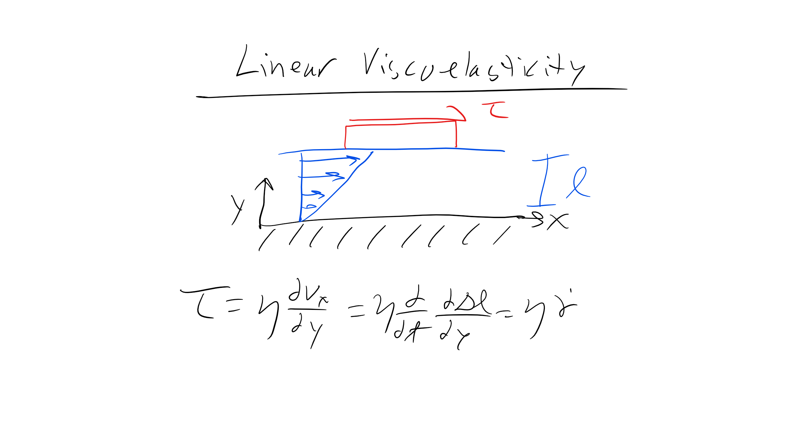
where \( \tau \) is shear force, \( \eta \) is viscosity, and \( \frac{d\gamma}{dt} \) is strain rate. Note that you can write this expression and re-derive it by considering the velocity profile as a function of y for a channel of length l, and you would obtain:

\[
\tau = \eta \frac{\partial v_{x}}{\partial y} = \eta \frac{\partial}{\partial t}\frac{\partial \Delta l}{\partial y} = \eta \frac{\partial \epsilon}{\partial t}
\]

You can think of this equation in the context of a channel filled with some fluid. When you apply a shear force to one plate, the plate will apply a shear force to the liquid. You'll notice that this equation has a very similar form to Hooke's law, but we replace strain with strain rate and Young's modulus with viscosity. We see that the faster the strain rate, the larger the resistive shear force, and the larger the viscosity, the larger the shear force. This makes sense, as pulling a plate through water is easier than pulling it through peanut butter. At very slow strain rates the shear force goes to zero, which is a property of liquids, whereas solids can be approximated as having infinite viscosity so they will not flow.

Thus if this were a liquid deformed under an applied shear stress there is no recovery when the shear stress is removed. But here this is linear because there is a proportional increase in \( \sigma \) and \( \frac{d\gamma}{dt} \) for some time or temperature. You can see this scenario schematically shown here.

When the viscosity is independent of strain rate or total strain, as is the case above, that material is Newtonian. Polymers, however, are typically non-Newtonian, i.e. viscosity is not a constant quantity but is dependent on strain rate or total strain. We can see an example in one of my favorite YouTube videos in the lecture slides. However, linear viscoelasticity is typically used to describe the mechanical response for polymers, glasses, tissues, and cells.

There are other types of interesting materials where the viscosity changes. For example, thixotropic materials will exhibit a decrease in viscosity as fluid flows—paints and fluidized granular beds are such examples. Rheopectic materials are those where viscosity will increase as the fluid flows, i.e. blood or printer ink.

Additionally, viscosity is yet another example of a material property that exhibits an Arrhenius temperature dependence:

\[
\eta = \eta_{0} e^{\frac{Q}{kT}}
\]

So we can clearly see here how the mechanical behavior of linear viscoelastic (LVE) materials is governed by both time and temperature, a common theme which will reappear over and over again.

Actually, let's take a step back and explore this concept a little bit by looking at one of the most common types of materials that behaves viscoelastically—those being polymers and other soft matter.

Time-Temperature Equivalence of Polymeric Materials

There is a well-defined difference in the Young's modulus between glassy, amorphous polymers and rubbery elastic polymers. Furthermore, we know that there is a temperature dependence for the Young's modulus. Below the \( T_g \) the modulus is very high, while at higher temperatures the modulus falls to that of a rubber. This relationship is typically drawn on a log(E) vs. log(T) plot where the several order of magnitude difference between the glassy and rubbery moduli is clear.

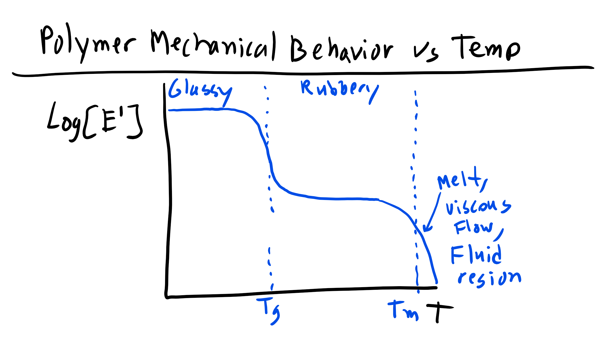
One other thing that must be noted is that at high temperatures, strictly amorphous polymers will have moduli that fall to zero; only crosslinked rubbers will maintain a non-zero modulus at high temperatures that is relatively invariant compared to the change between the amorphous and rubbery moduli. If there are no crosslinks, the polymer will simply flow irreversibly.

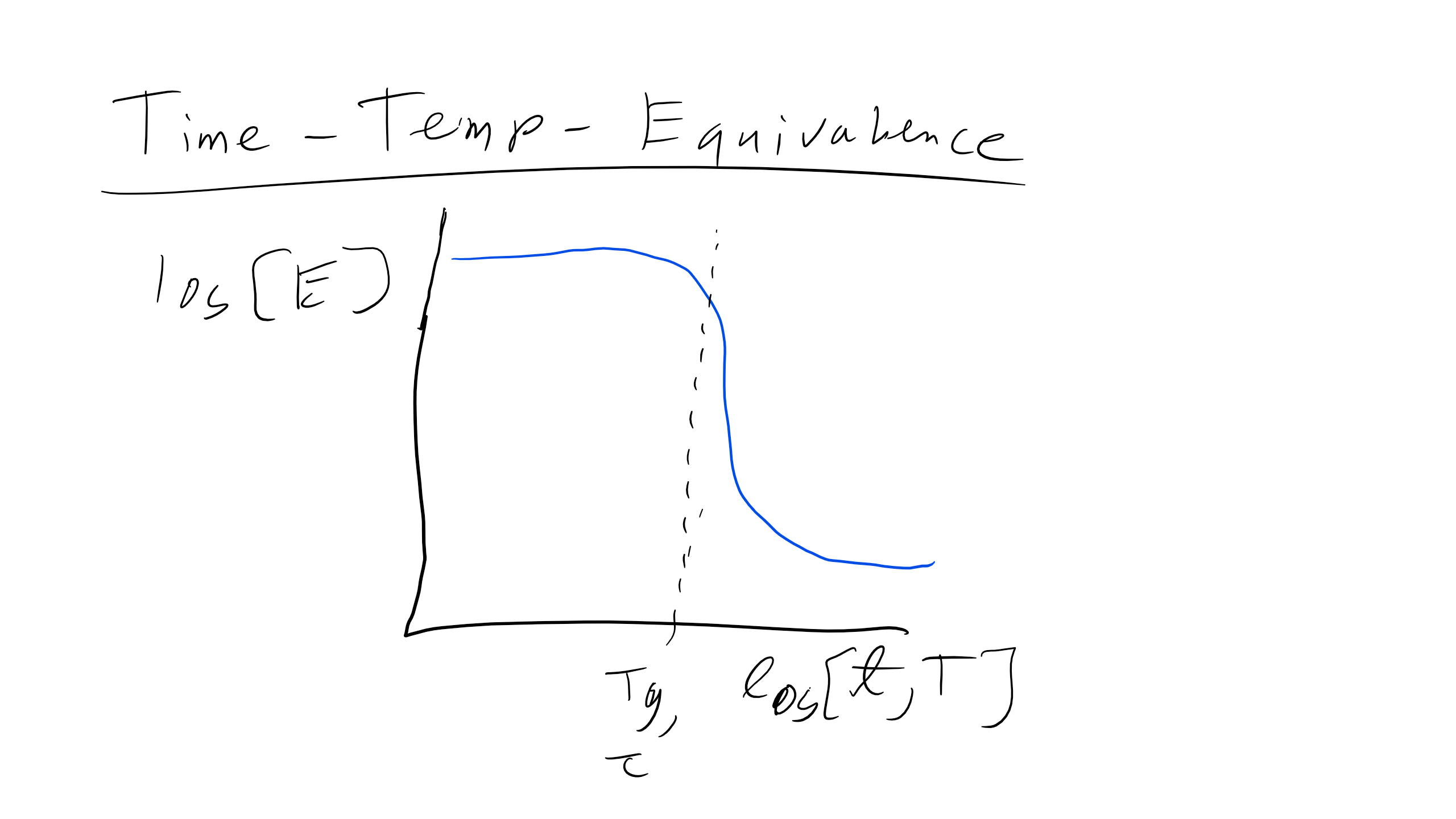
Now, if we remember back to the discussion of the glass transition, we said that the onset of glassy behavior is really due to the change in the characteristic relaxation time of a polymer, and how that relaxation time compares to the experimental time associated with a given stress effect. The glass transition would then be interpreted as changing the relaxation time with temperature, which molecularly could be understood as providing more (or less) thermal energy to overcome barriers to flow. However, we also said that if you change the timescale of the perturbation (e.g. deform a polymer really fast) you could obtain glassy behavior even without changing the temperature. This information leads us to believe that the modulus of a polymer is also time dependent, a fact that is borne out empirically. In fact, the graph of log(E) vs log(T) is qualitatively the same as the plot of log(E) vs. log(time), reflecting the origin of the glass transition.

In addition to changing the value of the Young's modulus, changing the timescale or temperature of an experiment can qualitatively change the shape of a stress-strain curve as well. For example, heating up a brittle, glassy polymer sample will decrease the Young's modulus but also increase the ductility of the sample, allowing longer elongations and more plastic deformation. There is thus a ductile-to-brittle transition where the polymer switches from undergoing stable plastic deformation (necking) to brittle failure; the exact temperature depends on the rate of testing and vice versa.

Finally, note that semi-crystalline polymers are characterized by a degree of crystallinity, which reflects the relative proportion of amorphous to crystalline regions. We would imagine that these regions could have very different moduli, especially above the glass transition temperature, and thus would expect the modulus to depend highly on the degree of crystallinity. This is indeed the case, and the modulus of semi-crystalline polymers has been observed to increase by a factor of over 100 as the degree of crystallinity increases. At low degrees of crystallinity, this change can be regarded as an increase in an effective crosslinking density for the amorphous regions, as the crystalline regions will likely bear very little load themselves. However, as the degree of crystallinity gets higher, the material can be more accurately regarded as a composite of a low modulus material and a high modulus material, a problem that is often treated in materials science.

Glass Transition Temperature

We have just discussed how non-crystalline amorphous polymers can be distinguished from semi-crystalline polymers based on the presence of long-range order. However, another critical parameter that is utilized to describe amorphous polymers is the glass transition temperature (\( T_g \)). Typically, non-crystalline polymers can be broadly classified as either rubbery or glassy, both of which exist as highly interpenetrated/entangled Gaussian coils at relatively high temperatures above the glass transition temperature.

When we say interpenetrated, the physical picture is of polymer coils that overlap with each other such that separate coils intertwine with each other. In this highly interpenetrated state, without solvent, the polymer acts as if it is unperturbed—that is, in the melt state the polymer is at the \( \theta \) condition, and can be treated as an ideal chain. You can think of melt polymers as essentially feeling some pressure due to surrounding polymers that overcomes excluded volume effects, yielding an ideal state. The ideal nature of polymers in the melt make them much easier to think about theoretically.

The glass transition temperature is the temperature at which a polymer transitions from its fluid-like state to a glassy state. When we say a glass, we mean a material with only short-range order but lacking the translational fluctuations associated with liquids. Hence it is like a solid, but with randomly positioned atoms rather than ordered ones as we expect in a crystal. We can identify the physical origin of the glass transition temperature in two different ways—first, you can think of increasing the temperature from below the glass transition, or you can think of decreasing the temperature from above the glass transition temperature. In either case, the glass transition is a competition between the available thermal energy \( kT \) and the strength of intermolecular bonds \( \epsilon_{ij} \).

If we think of increasing temperature, then the glass transition temperature is the point at which thermal energy is sufficient to break local intermolecular bonds, enabling fluid-like motions—that is, the point where \( kT > \epsilon_{ij} \). If we think of decreasing temperature, then the glass transition temperature is the point at which the viscosity of the polymer essentially becomes infinite, eliminating molecular motion. In either case, the key property of a glass is that the rearrangement of atoms is hindered, limiting the ability of the system to relax to equilibrium when a stress or perturbation is applied. This is intimately related to the concept of a characteristic relaxation time, which we will now discuss.

Relaxation Time \( \tau^* \)

The physical properties of amorphous polymers (and materials in general) are influenced by \( \tau^* \), the characteristic relaxation time of the polymer, and how large this relaxation time is relative to a relevant experimental time (or interaction time) \( t \). The relaxation time is essentially a measure of how long it takes for a material to return to equilibrium after the application of some perturbation. The ratio between the relaxation time and experimental time is called the Deborah number, \( De = \frac{\tau^*}{t} \). It is easiest to think of the importance of the relaxation time in terms of known material behavior.

Let's consider as an example a system consisting of some material in a container such that the material is attached to the container walls. We impose a perturbation on the system consisting of moving the walls of the container apart such that the material in the container is deformed or stretched.

First, consider the case that the relaxation time of a material is much smaller than the experimental time, such that \( \tau^* << t \) and \( De << 1 \). Because the relaxation time is so much lower than the experimental time, the material effectively relaxes instantaneously to the new system dimensions as the perturbation is applied; in other words, the system adjusts to the new constraint by relaxing to equilibrium immediately. Physically, we could imagine this as the material rearranging its constituent molecules to instantaneously fill the new volume of the container—we would say that the material flows, and call the material in the container a liquid.

Now consider the opposite case, where the relaxation time is much greater than the experimental time such that \( \tau^* >> t \) and \( De >> 1 \). Now when we adjust the walls of the container, the material effectively never relaxes to equilibrium as the perturbation occurs, instead being driven very far from equilibrium into a high-energy state. In our physical example, we would imagine the material in the container being stretched but being unable to adjust the positions of its atoms because the relaxation time is so long, so that the material instead builds up a large amount of strain energy; we would consider this an elastic response and call the material an elastic solid.

Note that the only distinction we are drawing here between the liquid and solid case is the experimental time—this implies that if we apply a stress or strain to a solid and wait long enough, it would appear to flow like a liquid. In the case of crystalline solids this would be due to the gradual movement of defects throughout the material to change the solid dimensions. In an intermediate regime where the relaxation time is roughly the same as the experimental time, the material will exhibit behavior consistent with both viscous liquids and elastic solids; we call these materials viscoelastic.

We can gain some understanding of relaxation times from the molecular structure of a given material. For example, for small molecules like water, the relatively free motion of water due to its small size would lead to a small relaxation time, and hence water is only solid at low temperatures. Polymers tend to exhibit a longer relaxation time due to the connectivity of monomers, requiring collective motion to adjust to a perturbation. As we will discuss shortly, at lower temperatures the energetic cost for this motion is too great to allow the polymer to flow, leading to glassy behavior. We might also imagine, then, that polymers with more rigid backbones have longer relaxation times due to the lessened flexibility of the chain.

Characterizing a polymer as a rubber, liquid, or solid (glass) is impossible without further information on the overall environment, as the response of the polymer depends on the time scales involved. We will also see that the relaxation time in polymers is a function of temperature, yielding many of the characteristic mechanical properties which we will discuss in future lectures. To wrap up: if the molecular motion is slow or hindered, the relaxation time of the polymer is very long and thus the polymer exhibits solid-like behavior.

Back to Glass Transition Temperature

A key point about the glass transition temperature is that it is not strictly a thermodynamic transition. The melting temperature, for example, results because there is some specific temperature for materials where the free energy of the liquid phase becomes lower than the free energy of the solid phase, leading to melting behavior (and more specifically there is an abrupt change in thermodynamic quantities reflecting a first-order phase transition). Hence, the melting point is thermodynamic in nature, resulting from the competition between the higher entropy liquid phase and lower enthalpy solid phase.

The glass transition, however, is not strictly thermodynamic, as a glass is not a stable thermodynamic phase but rather a kinetically trapped phase resulting from the large energy barriers faced by a glass when it must adjust to a perturbation. The glass transition thus reflects the kinetics and time scales of a system, and as such the transition temperature is not easily defined—in fact, the exact measurement depends on cooling rate, and typically a range of glass transition temperatures are reported for specific samples.

Free Volume Theory of \( T_g \)

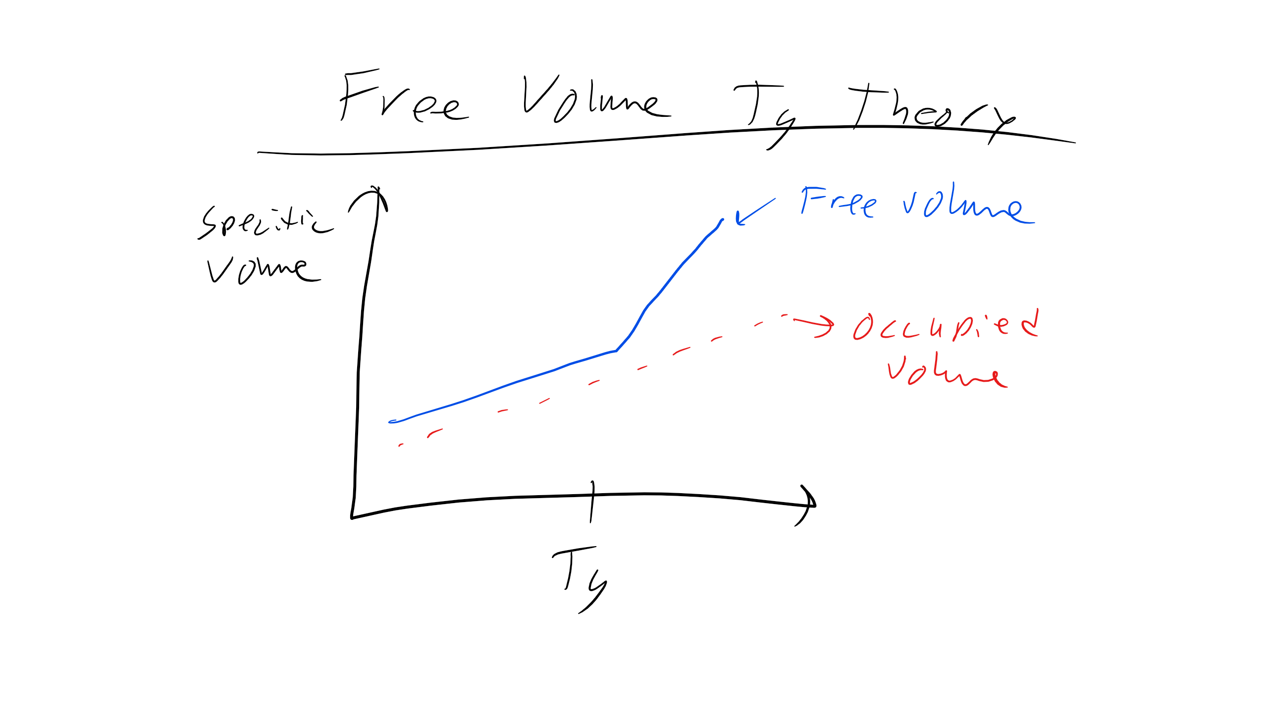
An explanation for the origin of the glass transition temperature comes from free volume theory. Free volume (not to be confused with excluded volume) is the space in a polymer sample in excess of the volume present in a random, densely packed glass. Free volume is the volume that monomers in a particular sample are able to access via thermal fluctuations. In a liquid state, we would imagine that the free volume is high, allowing large fluctuations and easy response to perturbations due to the availability of free volume through which monomers can move. By contrast, in the glassy state the free volume is very low and as a result molecular motion is hindered by steric or excluded volume considerations. The free volume is thus:

\[
V_F(T) = V(T) - V_0(T)
\]

where \( V_0 \) is the volume of a close-packed random glass (0.63), \( V \) is the actual volume of the sample, and \( V_F \) is the free volume. Note the temperature dependence of each term, which comes from thermal expansion governed by the thermal expansion coefficient:

\[
\alpha = \frac{1}{V}\frac{\partial V}{\partial T}
\]

As we gradually increase the temperature the volume available to the system will increase, reflecting increased fluctuations in monomer positions due to more available thermal energy.

Since the thermal expansion coefficient will be different between the glass and fluid states, \( V_F \) will increase with increasing temperature because the thermal expansion coefficient in the liquid state \( \alpha_l \) is greater than the thermal expansion coefficient \( \alpha_g \) in the glassy state (this controls the increase in \( V_0 \) with T). We can now write:

\[
V_F(T) = V_F(T_g) + (T-T_g)\frac{dV_F}{dT} \text{ for } T > T_g
\]

Dividing by \( V \) puts the right side in terms of the difference in thermal expansion coefficients and reduces all volumes to fractions of the total volume:

\[
f_F(T) = f_F(T_g) + (T-T_g)(\alpha_l - \alpha_g)
\]

\( T_g \) is then defined as the point where this fractional free volume falls below some critical value, and practically speaking can be found by looking at where the slope of the sample volume changes as a function of temperature (reflecting the change in expansion coefficient). Below the critical value, we can imagine the positions of the monomers are frozen due to the low volume available for monomer movements.

By this definition, polymers with greater free volume in the fluid state will experience a lower glass transition temperature, since you will have to decrease the temperature more to reduce the free volume fraction to the critical threshold. Qualitatively, this makes sense since if there is more free volume originally, it requires less thermal energy to access that volume, and so the glass transition temperature will be lower. This observation implies that the glass transition temperature will depend significantly on the molecular structure of the polymer. Finally, it has been shown experimentally that the critical fraction for the glass transition is fairly constant across many different molecules, making this analysis appropriate.

The glass transition temperature is also dependent on the rate of cooling of the sample. The cooling rate dependence of the glass transition temperature can be explained by what’s called percolation. If we imagine the polymer sample superimposed on a lattice, and each lattice point can be thought of as either in the glassy state or fluid state, then the network is percolated when a connected network of glassy points spans the entire lattice. In other words, it is not necessary for the entire polymer sample to be glassy; it is only necessary for connected regions that cross the network to be glassy, since these connections essentially cut off the fluid parts from each other, leading to glassy behavior on the macroscale.

We can think of each lattice point as transitioning between fluid and glassy with some characteristic probability, and can also imagine some other characteristic probability for the point to transition from glassy back to fluid. Physically, this reflects the ability of monomers to move through the available free volume, and hence at lower temperatures we expect the probability of a fluid-to-glass transition to increase, and the probability for a glass-to-fluid transition to decrease as the decreasing free volume favors the glassy state.

As we cool the sample, then, the probability of forming a glass progressively becomes higher, and the time taken for glass points to transition back to fluid takes progressively longer. If we cool at a very fast rate, lattice points will have sufficient time to transition from fluid to glass but not back (since as we cool it takes longer and longer for the glass-to-fluid transition), leading quickly to a percolated network at a high temperature since glassy behavior will be observed as soon as connected glassy regions span the sample. If we cool at a slower rate, a percolated network is more difficult to form because at higher temperatures the relatively short time associated with the glass-to-fluid transition will disrupt the network as it forms. This means that the glass transition will be observed at a lower overall temperature.

Tg and Chemical Structure of Monomers

Trends in \( T_g \) can be explained by looking at the chemical structure of monomers due to the influence of monomer structure on both chain flexibility and free volume. Recall that \( T_g \) is determined by the onset of long-range cooperative molecular motion, meaning the motion of 10–30 connected chain monomers at once. The cooperative motion requires both sufficient thermal energy to induce the movement of these monomers and sufficient free volume for the monomers to move into. Both of these requirements are influenced by monomer structure. There are essentially three elements of monomer structure that can influence these motions:

1. Chain interactions – energetic interactions between monomers
2. Ease of rotation about main chain bonds – whether there is significant steric hindrance to rotation
3. Amount of free volume available – how densely the monomers pack

We can think of polymers as essentially divided into their backbone and sidechains coming from that backbone. In polymers with flexible backbones, like polyethylene (lots of C–C single bonds) and PDMS (Si–O bonds, which are flexible due to the 4 electrons on the oxygen atoms in place of hydrogens), the hindrance to rotation is low and hence less thermal energy is necessary to induce molecular motion, leading to a low \( T_g \).

On the other hand, polymers with phenyl molecules along the backbone (e.g. polycarbonate) tend to have a much higher \( T_g \), since the bulky phenyl constituent greatly increases the amount of energy necessary for rotation (i.e. the rigidity). Note that we can generally relate \( C_\infty \) to the rigidity of a backbone, and hence expect \( T_g \) to increase with \( C_\infty \).

Similarly, large bulky sidechains, such as phenyl groups, also oppose rotation due to steric hindrance, and in addition decrease the amount of free volume available since they occupy a greater excluded volume, leading to a higher glass transition temperature. Finally, intermolecular interactions, such as hydrogen bonds or ionic interactions, which are typically seen between sidechains, will tend to greatly increase the glass transition temperature since thermal energy will also have to break these bonds to induce rotation.

The lecture notes provide some examples of polymers, sidechains, and the related \( T_g \) values. The main principles to keep in mind are that chain flexibility allows easier cooperative movement of monomers, decreasing the \( T_g \), and increased free volume around the chain backbone lowers the barrier to cooperative movement and hence decreases the \( T_g \).

We can also relate these observations back to the idea of crystallinity, as well, as the factors that influence the glass transition temperature will also influence the ability of polymers to crystallize. In fact, there is a correlation between \( T_g \) and \( T_m \) for semi-crystalline polymers — typically \( T_g \) is about 0.5 to 0.8 \( T_m \) in Kelvin.

Spring and Dashpot Models

One of the most common ways to model and conceptualize the idea of linear viscoelasticity and to recreate the mechanical behavior that we just saw is to build spring–dashpot models. The time-dependent mechanical behavior can be represented by a spring–dashpot model. The dashpot is essentially just a plunger in a cylinder of fluid while the spring is essentially a spring.

The mechanical response of the spring is Hookean and represents an elastic response. The spring is described by the following equation:

\[
\sigma_{s} = E_{s}\epsilon_{s}
\]

where \( \sigma_{s} \) is the stress in the spring, \( E_{s} \) is the stiffness of the spring, and \( \epsilon_{s} \) is the strain in the spring.

The mechanical response of the dashpot is a viscous, time-dependent response (we are at a constant temperature) and we can describe it as:

\[
\sigma_{d} = \eta_{d} \dot{\epsilon_{d}}
\]

where \( \sigma_{d} \) is the stress in the dashpot, \( \eta_{d} \) is the viscosity of the dashpot, and \( \dot{\epsilon_{d}} \) is the strain rate of the dashpot.

Now, when we connect these components in series, parallel, or some other combination we can model certain LVE material mechanical behaviors phenomenologically. Let's take a look at one such model, the Maxwell Model.

Maxwell Model

Let's take a look at the Maxwell model, which is a combination of a spring in series with a dashpot that contains a Newtonian fluid.

Now let's say that we stress the system with some applied stress \( \sigma_M \). In this configuration, the stresses will be the same for the spring and the dashpot as they are arranged in series; however, the strains in the dashpot and the spring will be different, which gives us the following relationships:

\[
\sigma_{M} = \sigma_{s} = \sigma_{d}
\]
\[
\epsilon_{M} = \epsilon_{s} + \epsilon_{d}
\]
\[
\dot{\epsilon_{M}} = \dot{\epsilon_{s}} + \dot{\epsilon_{d}}
\]
\[
\dot{\epsilon_{M}} = \frac{\dot{\sigma_{M}}}{E} + \frac{\sigma_{M}}{\eta}
\]

This last expression is the constitutive equation for the Maxwell Model.

With this system we can do two types of experiments: stress relaxation (\( \epsilon = \epsilon_{0} \), i.e. constant strain) and creep (\( \sigma = \sigma_{0} \), i.e. constant stress).

For stress relaxation we can plug into our equation and solve for how the stress in our Maxwell model should vary over time:

\[
0 = \frac{1}{E}\frac{d\sigma}{dt} + \frac{\sigma}{\eta}
\]
\[
\int^{\sigma}_{\sigma_{0}}\frac{d\sigma}{\sigma} = \int^{t}_{0}\frac{-E}{\eta}dt
\]
\[
\sigma(t) = \sigma_{0}\exp\left(\frac{-Et}{\eta}\right)
\]
\[
\sigma(t) = \sigma_{0}\exp\left(\frac{-t}{\tau}\right)
\]

where \( \tau = \frac{\eta}{E} \) is the relaxation time. Here we predict that the stress will decay to zero, which is in disagreement with the way many viscoelastic materials behave—they must retain some stress.

Similarly for creep:

\[
\frac{d\epsilon}{dt} = 0 + \frac{\sigma_{0}}{\eta}
\]
\[
\int^{\epsilon}_{\epsilon_{0}}d\epsilon = \int^{t}_{0}\frac{\sigma_{0}}{\eta}dt
\]
\[
\epsilon(t) = \epsilon_{0} + \frac{\sigma_{0}t}{\eta}
\]

This result does not give us the glassy–viscoelastic–rubbery transition we expected to see.

Kelvin-Voigt Model

There is also the Kelvin-Voigt (KV) model, which has the spring and dashpot arranged in parallel.

In this case, the strain is the same, because they are in parallel, but now the stresses are different, so we get:

\[
\epsilon_{KV} = \epsilon_{s} = \epsilon_{d}
\]
\[
\sigma_{KV} = \sigma_{s} + \sigma_{d}
\]
\[
\sigma_{KV} = E_{s}\epsilon_{s} + \eta_{d}\dot{\epsilon_{d}}
\]
\[
\dot{\epsilon_{KV}} = \frac{\sigma_{KV}}{\eta_{d}} - \frac{E_{s}}{\eta_{d}}\epsilon_{KV}
\]

Again, this last expression is the constitutive equation for the KV model.

Now for stress relaxation we get the final equation for stress versus time as:

\[
\sigma(t) = E\epsilon_{0}
\]

The KV model is particularly bad here, where the model predicts an infinite spike in stress and then a time-independent stress afterwards.

For creep we get:

\[
\epsilon(t) = \frac{\sigma_{0}}{E}\left[1-\exp\left(-\frac{t}{\tau}\right)\right]
\]

Here again the KV model does not give a transition from glassy to viscoelastic, and then again to rubbery.

Now, as you can see, the Maxwell and KV models are not very realistic, in particular the stress relaxation for the KV and the creep expression for Maxwell. A better model would be the Standard Linear Solid Model.

Standard Linear Solid Model

You can now build even more complex combinations to model viscoelastic properties, like the Standard Linear Solid Model or Maxwell-Zener Model, which combines both models to better capture the behavior of viscous materials—and there are many more complex models as well to represent the behavior of materials.

Here we can see that we have a spring in series with our KV model. We know that for parallel components we will add stress and the strains will be equivalent, whereas for series components we will add strains and stresses will be equivalent. So for the total system we will find that:

\[
\epsilon_{SLS} = \epsilon_{KV} + \epsilon_{1}
\]
\[
\sigma_{SLS} = \sigma_{KV} = \sigma_{1}
\]

where SLS indicates the entire model, KV indicates the KV arm, and 1 indicates the spring.

Now we can start to write some expressions below:

\[
\dot{\epsilon_{SLS}} = \dot{\epsilon_{KV}} + \dot{\epsilon_{1}}
\]
\[
\dot{\epsilon_{SLS}} + \epsilon_{SLS}\frac{E_2}{\eta} = \frac{\sigma_{SLS}}{\eta}\left(1 + \frac{E_2}{E_1}\right) + \frac{\dot{\sigma_{SLS}}}{E_1}
\]

This model is much better, as we obtain an exponential response for both creep and stress relaxation. However, these are just models and give poor numerical results, but the general trends are very consistent. There are infinite models that can be built with increasing complexity, as seen below.

Boltzmann Superposition Principle and Creep Compliance

Another approach that can be taken to modeling creep and stress relaxation is by leveraging the fact that stress and strain are linearly related at a given time and temperature. As this is true, we can use the Boltzmann superposition principle to determine the stress by summing the strain during multiple deformation steps and defining a parameter called the creep compliance \( J(t) \), which relates strain to stress as a function of time:

\[
\epsilon(t) = J(t)\sigma
\]

You essentially treat each loading step as making an individual contribution to the final deformation, and you can obtain the final deformation by simply summing each contribution, i.e.:

\[
\epsilon(t = t_n) = \Delta\sigma_1(t_n - t_1) + \Delta\sigma_2(t_n - t_2) + \Delta\sigma_3(t_n - t_3)
\]

You can do the same procedure for stress relaxation, but you have to define the stress relaxation modulus \( G(t) \).

Dynamic Mechanical Testing

The more utilized characterization technique is instead dynamic mechanical testing to probe the viscoelastic behavior of materials. In this experiment the polymer is subjected to a sinusoidal loading at variable frequencies which can be described as:

\[
\sigma_{applied} = \sigma_0 \sin \omega t
\]

This is the applied stress, but remember we are dealing with a viscoelastic material so there will be a phase lag, \( \delta \), in the strain behavior which will also be sinusoidal:

\[
\epsilon = \epsilon_0 \sin \omega t
\]

So what we will end up with is that the material will actually experience a stress that contains the phase lag as shown below:

\[
\sigma = \sigma_0 \sin(\omega t + \delta)
\]
\[
\sigma = \sigma_0 \sin \omega t \cos \delta + \sigma_0 \cos \omega t \sin \delta
\]

In the equation above, the first term represents the component that is in phase with the strain or the elastic response, while the second term represents the out-of-phase behavior or the viscous response. We can then define two elastic moduli to describe the in-phase and out-of-phase behavior. The storage or elastic modulus is the in-phase contribution and is defined as:

\[
E' = \frac{\sigma_0 \cos \delta}{\epsilon_0}
\]

and the loss modulus is the out-of-phase component and is defined as:

\[
E'' = \frac{\sigma_0 \sin \delta}{\epsilon_0}
\]

We can now re-write our expression for the stress in the material as:

\[
\sigma = E' \sin \omega t + E'' \cos \omega t
\]

then by definition we have that:

\[
\tan \delta = \frac{E''}{E'}
\]

This is sometimes called the loss tangent and essentially represents the amount of energy lost over the energy stored. You might also see these expressions written using complex variables like so:

\[
\epsilon = \epsilon_0 e^{i \omega t}
\]
\[
\sigma = \sigma_0 e^{i (\omega t + \delta)}
\]
\[
E = \frac{\sigma_0}{\epsilon_0} e^{i \delta} = \frac{\sigma_0}{\epsilon_0} (\cos \delta + i \sin \delta) = E' + iE''
\]

Analysis of Dynamic Mechanical Testing Experiments

Typically you will find, at a fixed temperature, that the loss tangent and the loss modulus are very small at both very low and very high frequencies and they will typically peak at intermediate frequencies. The storage modulus is high at high frequencies (short times), which should make sense intuitively as polymers will typically behave glassy or elastic at high frequencies and short times (strain rate is faster than the relaxation time of the polymer). At low frequencies (long times, longer than the relaxation time), the polymer will behave more like a viscous fluid.

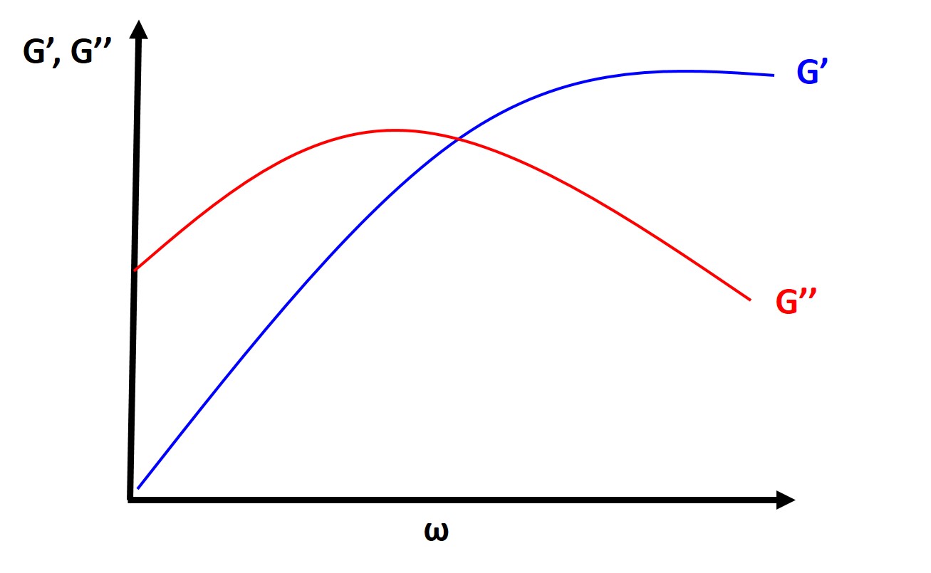
More importantly, from this analysis we can determine experimentally the characteristic relaxation time from the point where \( G' \) and \( G'' \) intersect.

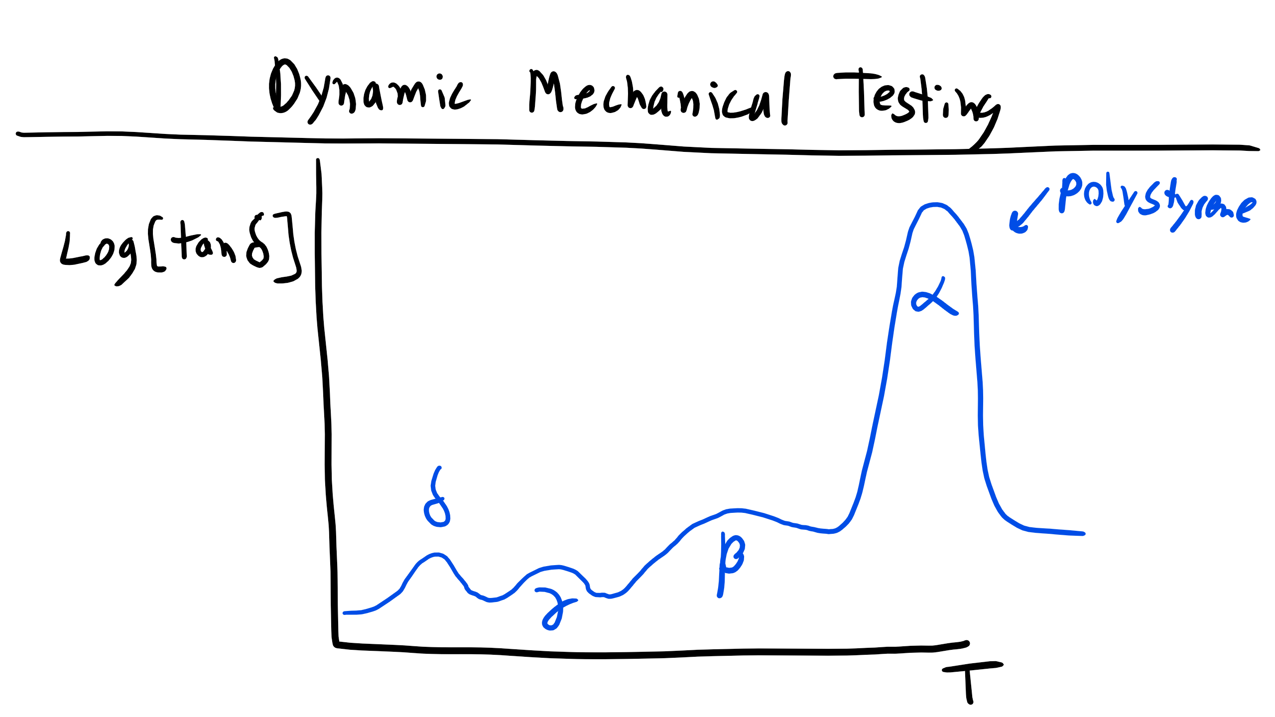
More often we will find that typical DMA experiments plot \( G' \), \( G'' \), and \( \tan \delta \) as a function of temperature. Here you will typically see larger peaks and changes in these parameters, as we have already seen that the modulus of polymers is temperature dependent. Alternatively, as we have already discussed at length, the temperature will affect the amount of molecular motion and free volume, which will increase and affect these properties, particularly the loss tangent. So you will expect to see large changes at the glass transition temperature and melting temperature, but you might also expect to see other small peaks associated with secondary transitions (note this is not referring to second-order thermodynamic transitions like \( T_g \), this is just referring to the magnitude of the peaks) associated with molecular motion of the polymer, such as the temperature at which backbone side group rotation is accessible.

As you can see in the figure, the primary observable and measurable change in the storage modulus occurs when you pass through \( T_g \). However, the more subtle difference in behavior can be found in the variation of the loss tangent as a function of temperature. Here we can see multiple different peaks at different temperatures with varying amplitudes. In these plots each peak is typically labeled \( \alpha, \beta, \gamma \), etc., in order of descending temperature. In this graph the \( \alpha \) peak or relaxation corresponds to the \( T_g \) in an amorphous polymer or it could be \( T_m \) for a semi-crystalline polymer. The \( \beta \) peak here corresponds to cooperative motion of segments of the main chain. The \( \gamma \) peak is due to phenyl group rotation around the backbone, and the \( \delta \) peak has been linked to some wiggling of the phenyl group most likely due to defects or tacticity differences.

For semi-crystalline polymers this analysis can become even more difficult because of the microstructure of spherulites. This makes it very difficult to separate the amorphous and crystalline behavior. One example of this can be seen for LDPE and HDPE. You can see some similar transitions (i.e. \( \gamma \)) but also stark differences. The primary difference between LDPE and HDPE is the amount of branching, which is much larger in LDPE than in HDPE. Here the \( \alpha \) and \( \alpha' \) peaks are associated with motion in the crystalline regions, while the \( \gamma \) peak is associated with the amorphous region. Finally, the \( \beta \) relaxation is associated with the motion of the branches.

Now, the analysis of these peaks in polymers is a great source of debate, but when analyzing them just make a reasoned argument thinking about the thermal energy required for a particular type of motion.

Time-Temperature Equivalence

For viscoelastic polymers there is a theoretical equivalence of time and temperature. We have seen previously that a polymer can exhibit glassy or rubbery behavior by changing either the temperature or the strain rate, i.e. time. So we can establish the principle of time-temperature superposition, or the theoretical equivalence between changing the timescale or temperature of an experiment.

An experimentally derived equation relating these two quantities, known as the WLF equation, was found by noticing that you can superpose curves by keeping one curve fixed and shifting all the others by different amounts horizontally parallel to the logarithmic time axis. We can take a reference temperature point, \( T_s \), and a temperature point, \( \tau_s \), in order to fix one curve. We then have to find the \( \tau \) for a new curve with the same compliance as our reference curve at \( T_s \). The amount of shift will then simply be \( \log \tau_s - \log \tau \), which we will define as our shift factor:

\[
\log a_T = \log \tau_s - \log \tau = \log \frac{\omega_s}{\omega}
\]

[Figure: WLF Time-Temperature Superposition.]

With this, Williams, Landel, and Ferry (WLF) empirically fit these polymer curves and found the following empirical equation:

\[
\log a_T = \frac{-C_1 (T - T_s)}{C_2 + (T - T_s)}
\]

where \( C_1 \) and \( C_2 \) are empirical fitting constants, 17.44 and 51.6 K respectively, if one chooses \( T_s = T_g \). This equation was later re-derived using theory based on free volume, akin to the theory for the glass transition, reflecting similar physical origins. The derivation is beyond the scope of this lecture (and you are probably sick of derivations at this point), but you can read it in Young and Lovell, Chapter 5. The resulting equation is:

\[
\log a_T = \frac{-(B / 2.303f_g)(T - T_g)}{f_g / \alpha + (T - T_g)}
\]

where \( f_g \) is the fractional free volume at the glass transition temperature and \( \alpha \) is the volumetric thermal expansion coefficient. Typically for polymers, \( f_g = 0.025 \) and \( \alpha = 4.8 \times 10^{-4} \, K^{-1} \). \( B \) is another fitting constant.

Limitations of WLF

The WLF equation is applicable to homogeneous, linear viscoelastic materials that are isotropic and amorphous. They must be in the temperature range \( T_g \) to \( T_g + 100^{\circ}C \).