Chapter 1: Introduction to Materials, X-Ray Diffraction, and Inter and Intramolecular Bonding

1.1 Topics Covered in this Book

• Part I: Bonding, Structure, Defects, and Phase Diagrams
• Part II: Mechanics of Materials
• Part III: Electrochemistry, Electrical, and Optical

I have recorded a series of recorded video lectures to supplement this text which can be viewed in the playlist here:

https://www.youtube.com/playlist?lis...5J4dxGKE5Wgkrk

1.2 The Materials Tetrahedron

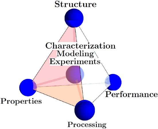
The four corners of the Materials Science and Engineering Tetrahedron are: Structure, Processing, Properties, Performance. At the center is a combination of Charact/Modeling/Exp.

A couple of quick examples if you process sheet metal by cold rolling you change the structure and induce more dislocations in the material. This in turn will change the yield strength (property) and thus the performance of that sheet metal in the application of interest. As materials scientists at the core of what we do is try to characterize material with experimentation and simulation to better understand this materials tetrahedron and to eventually reach a point where we can begin to predict some material responses.

Any other examples where we can apply this materials tetrahedron?

• Lead Titanate
• Cold Rolling Titanium Sheet
• Cross-Linked Rubber or Kevlar

Different Types or Classifications of Materials:

• Metals
• Polymers
• Ceramics
• Composites
• Active Matter
• Piezoelectric
• Shape Memory Alloys
• Ferromagnetic Materials

Material Properties:

• Mechanical
• Thermal
• Magnetic
• Optical
• Electrical
• Structure

1.3 Atomic Structure and Bonding:

Before diving into materials structure, we need to start at the basics and build up from the subatomic to atomic, nano, micro, and then macrostructure. So hopefully we all remember from our chemistry classes...

An atom is compose of a nucleus of protons and neutrons. A cloud of electrons surrounds the nucleus. The atomic number of an element is denoted by the number of protons in the nucleus. Atomic mass is the sum of the masses of proton and neutrons. Atomic weight of an element is the weighted average of the atomic masses. The atomic mass unit (amu) is defined as \(\frac{1}{12}\) the atomic mass of Carbon 12.

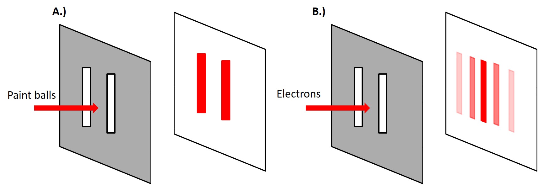
When we discuss the different types of bonding we are typically interested in the electronic structure of an element or a material. In particular, we are interested in the valence electrons or the outermost electrons. Now electrons have particle-wave duality, i.e. electrons are governed by quantum mechanics. The classical example being the double slit experiment. It was conducted by Thomas Young in 1801 where he showed that light and later Davisson and Germer demonstrated that electrons display an interference pattern when shot at a double slit. This is because electrons can behave like particles and waves and when a wave passes through a double slit there will be constructive an destructive interference of the waves.

This is phenomenon is particularly relevant to X-Ray Diffraction (XRD). This is a technique we will use in our first lab to investigate the atomic structures of several different materials. In general, diffraction will occur when a wave encounters a series of regularly spaced obstacles or slits that are capable of scattering the wave and have spacings that are comparable to the magnitude of the wavelength of the indecent wave.

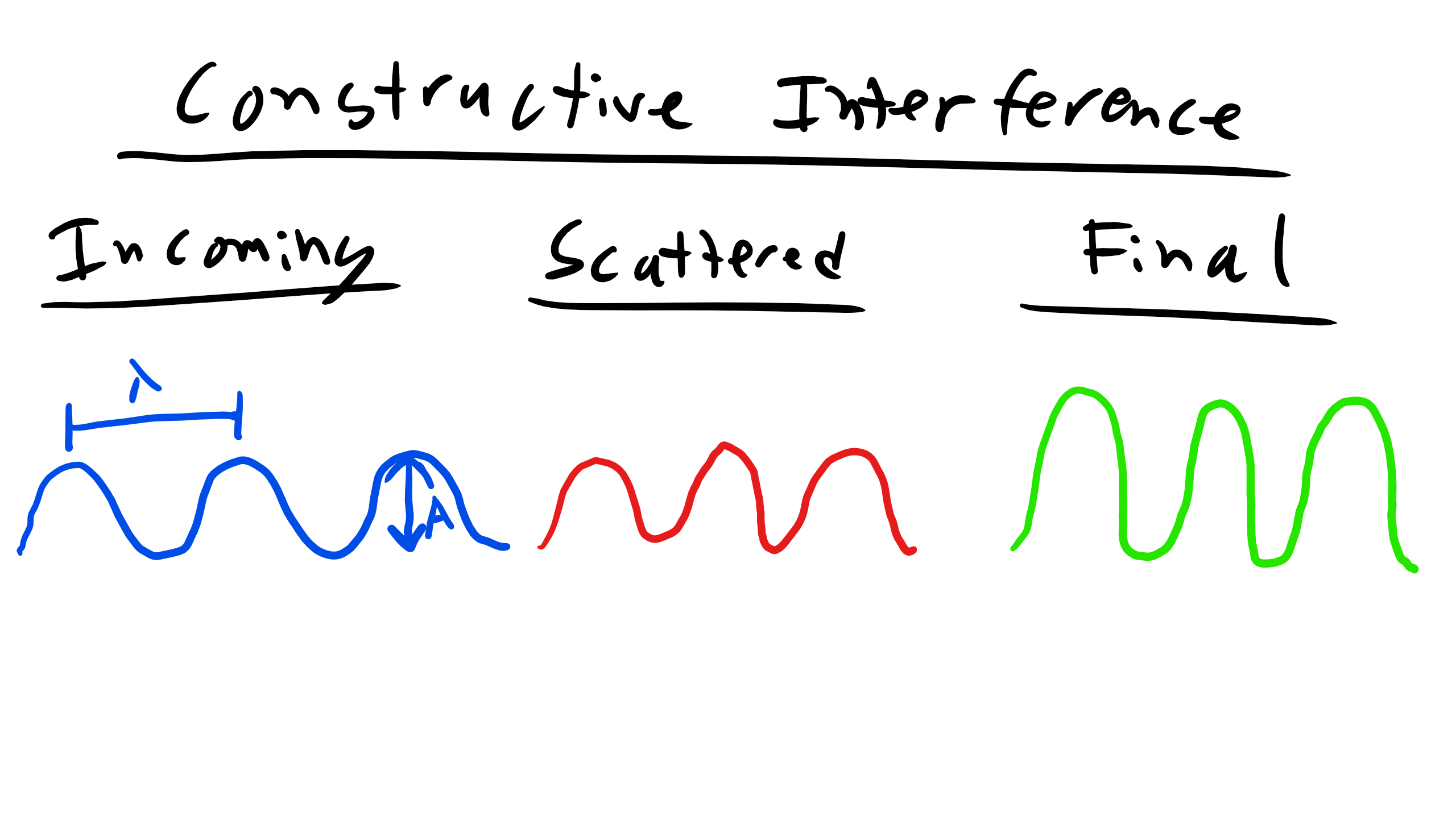
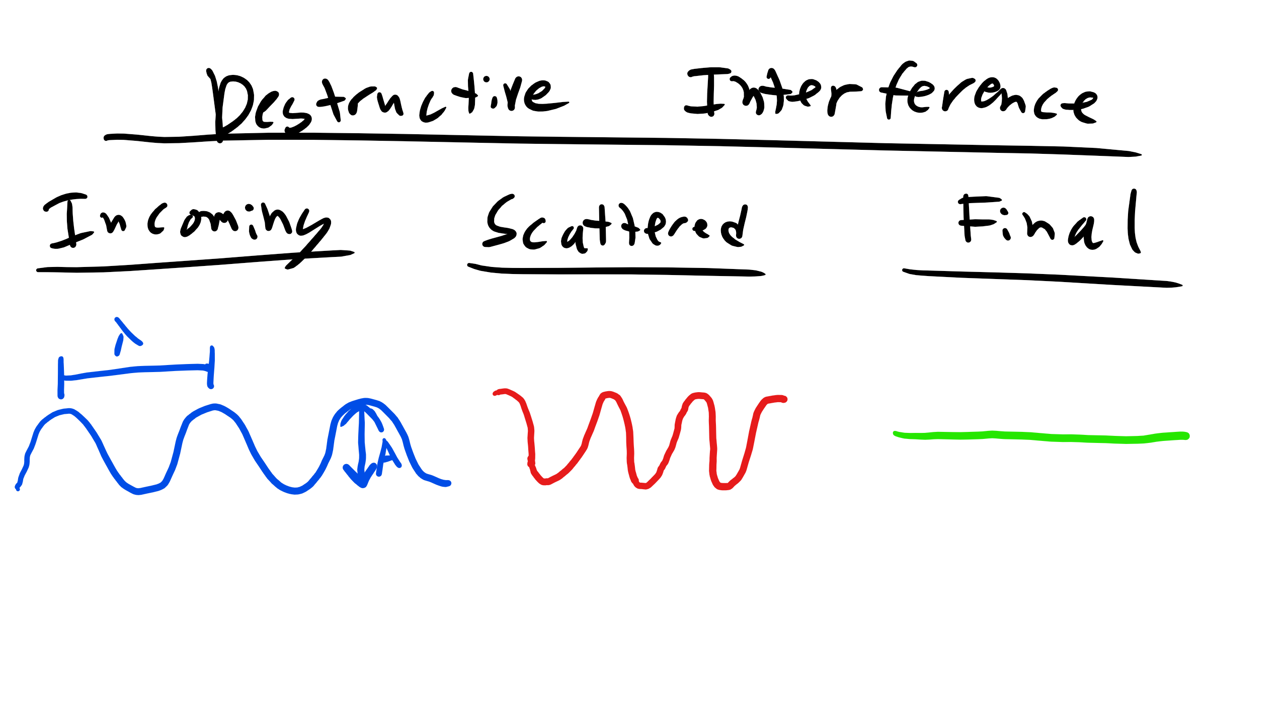
Let's look at an example of constructive vs. destructive interference as seen below. Consider the first set of waves that are incident to the scattering event. After they pass through the scattering event you see that the waves are still in phase so the resultant waves constructively interfere with each other and produce the resultant diffracted wave that is now twice the amplitude . We previously assumed that the two incident waves were both of the same magnitude and wavelength. Conversely for destructive interference after the waves encounter the scattering event they are out of phase which results in the waves canceling each other out or in other words destruction.

1.3.1 Bragg Diffraction

Sir William Lawrence Bragg was a very brilliant scientist and he won the Nobel Prize for Bragg Diffraction when he was 25 and he won it with his father. Bragg realized that if we want to deduce material structure we can actually investigate this with X-rays. Cu-K\(_{\alpha}\) radiation has a wavelength of 1.542\(\AA\). This is on the order of the spacing of atomic structures which meets one of our criterion for diffraction and crystal structures are made of regularly spaced obstacles for which a beam of X-rays can scatter. Bragg saw that in doing so it would be possible deduce the inter-atomic or inter-planar spacing between atoms for a given incident wavelength . Look at 2D schematic below

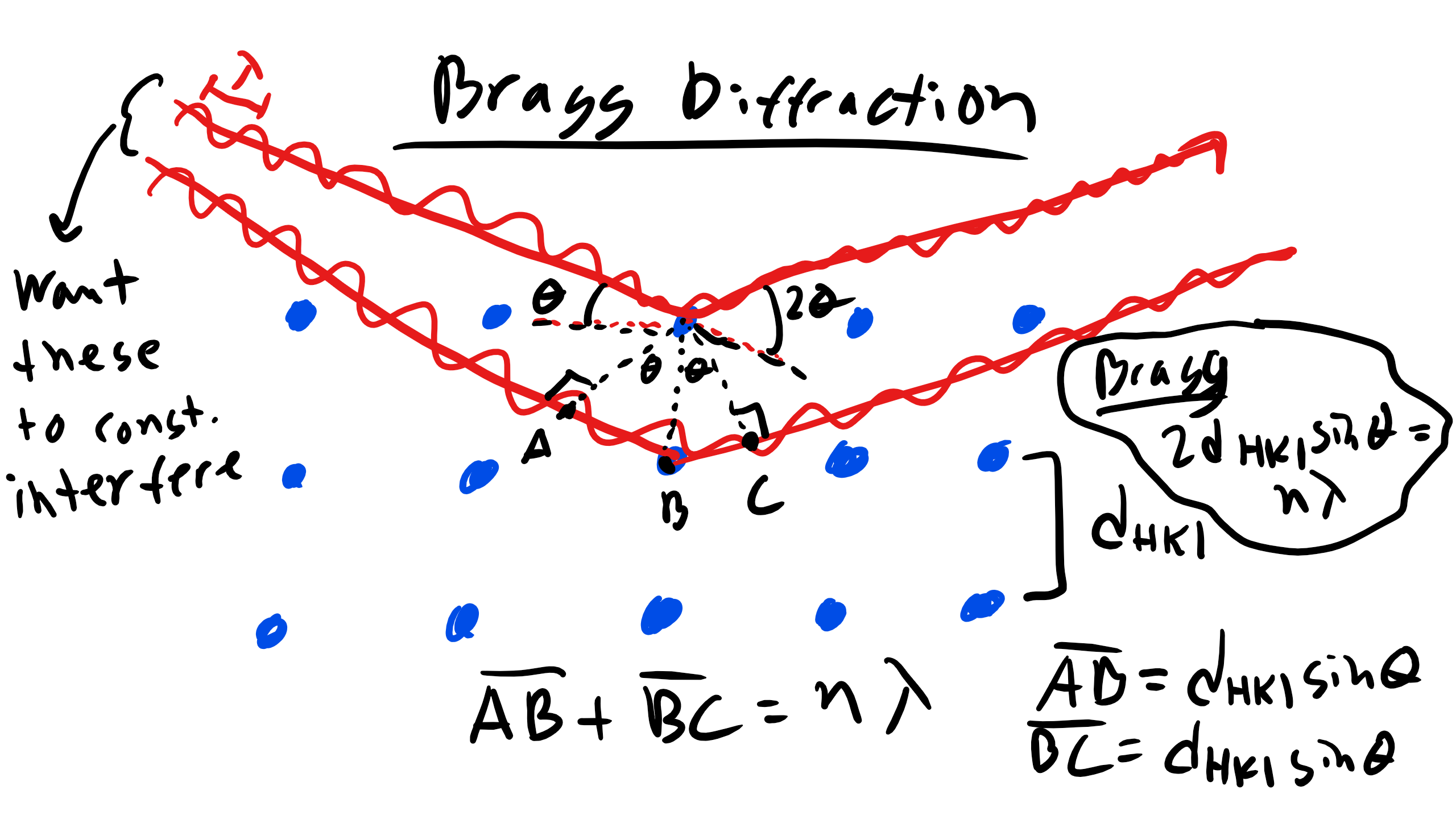
We again have two incident beams that will interact with two planes of atoms each at an angle of incidence \(\theta_{B}\) which is the Bragg angle or the condition for diffraction. So what is the condition for diffraction in the example? Well we have to have constructive interference so the extra path length traveled by the lower incident wave must be equal to an integer number of wavelengths as the upper incident wave and that equivalence gives us Bragg's Law

\begin{equation}
n \lambda = 2d_{hkl} \sin \theta_{B}
\end{equation}

where n is an integer number which denotes the order of reflection, \(\lambda\) is the wavelength, \(\theta_{B}\) is the Bragg angle, and \(d_{hkl}\) is the interplanar spacing.

The interplanar spacing for cubit materials is defined as

\begin{equation}
d_{hkl} = \frac{a}{\sqrt{h^2 + k^2 +l^2}}
\end{equation}

where a is the lattice parameter of the unit cell, and h,k, and l are the miller indices. More on these much later in the Structure Lecture.

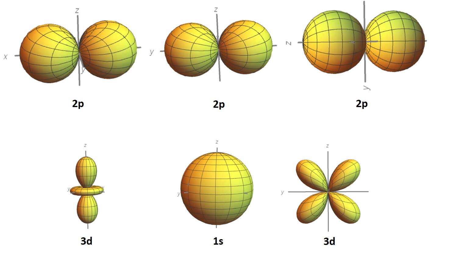
But now back to electrons... Electrons are described by quantum numbers, specifically 4 quantum numbers. The principal quantum number, n, specifies the electron shell which takes on integer values, sometimes designed by K, L, M, N, O which corresponds to n = 1, 2, 3, 4, 5.... Remember back to chemistry that these shells correspond to the Bohr atomic model where electrons revolve around discrete orbitals and that the electrons are quantized in discrete energy states. In reality it is not a discrete orbital but instead electrons reside within some cloud according to a probability distribution. The second quantum number sometimes referred to as the aziumuthal quantum number, l, designates the subshell. l is an integer value as well and defined as l = 0 to l = (n-1). The letter designation is s, p, d, and f respectively. cite The orbital shapes depends on l.

The number of electron orbitals for each subshell} is determined by the third quantum number sometimes called the magnetic quantum number, \(m_{l}\). \(m_{l}\) can take on integer values between -l and +l. Additional with each electron there is a spin moment which must be oriented either up or down and this is captured by the fourth and final quantum number \(m_{s}\).

We fill electron orbitals or states using the Pauli exclusion principle, each electron state can hold no more than two electrons and just have opposite spins. When electrons are occupying states such that the energy is minimized they are in the ground states but there are times when the electrons can become excited and transition to higher states.

1.4 Types of Bonding: Covalent, Ionic, Metallic, and Van Der Waals

Elements that have no valence electrons or that have a completely filled outer shell are called the inert or noble gases. All other elements which do not have a completely filled outer shell have valence electrons and these electrons are the ones of import when it comes to bonding.

Bonding is critically important as most of the structural, physical, and chemical properties are influenced or determined by the interatomic bonding. And typically we are concerned with four types of bond.

1. Covalent (5eV or about 200 kT)
2. Ionic (1-3eV or 80kT)
3. Metallic (0.5eV or 20kT)
4. Van Der Waals (0.001-0.1eV or 0.2kT )

First question why do we even need bonding? Or a better question why does bonding occur?

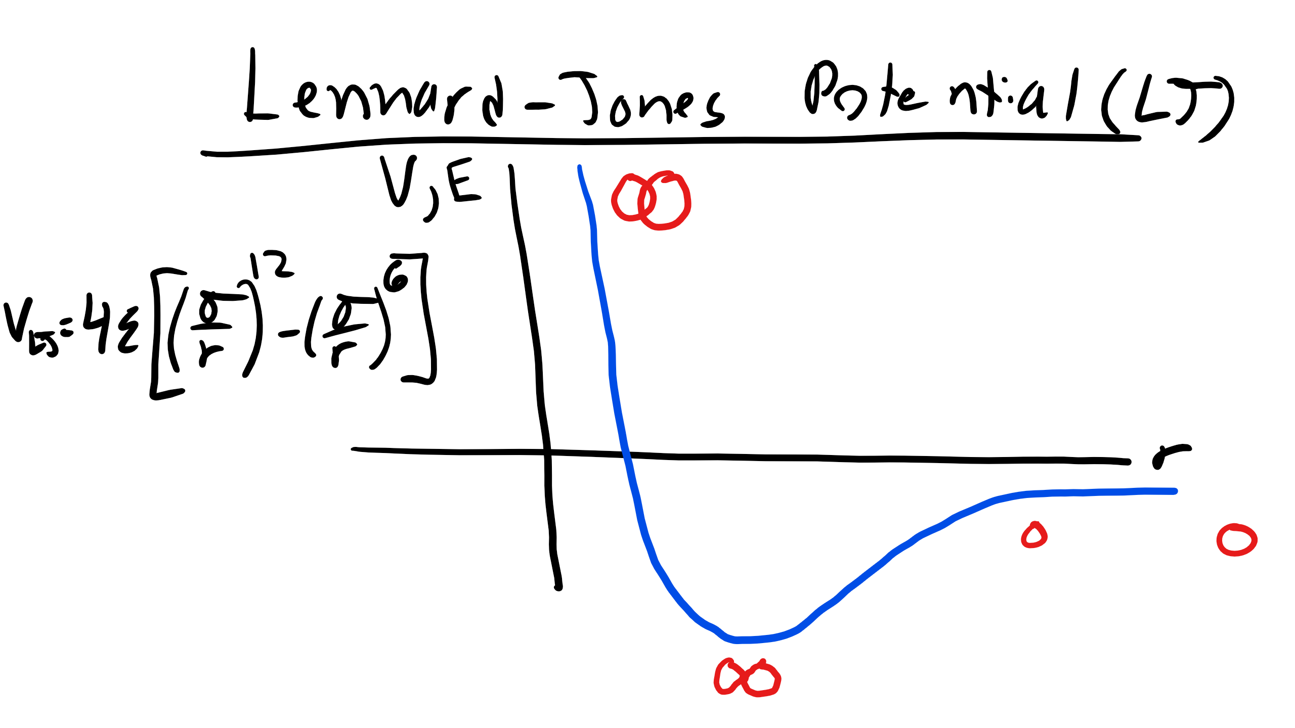
Well it all goes back to Gibbs, the energy of the set of bonded atoms is lower than the isolated atoms. There are forces of attraction and repulsion between electrons and protons. And we remember that the force (F) is related to the potential energy (U) by \(F = - \nabla U\). Remember that \(\nabla\) is the gradient mathematical operator and will take the partial derivative of the function with respect to the dimensionality of the problem. Now there are many different equations or potentials that describe the interactions between atoms i.e. Morse, Born-Mayer, Van Der Waals, etc. Let's take a look at one of these potentials, the Lennard-Jones (LJ) Potential which approximates the interaction between a pair of neutral atoms (it is popular due to the computational simplicity)

\begin{equation}
V_{LJ} = 4\epsilon \bigg[\bigg(\frac{\sigma}{r} \bigg)^{12} - \bigg(\frac{\sigma}{r} \bigg)^{6}\bigg] = \epsilon \bigg[\bigg(\frac{r_{o}}{r} \bigg)^{12} - 2\bigg(\frac{r_{m}}{r} \bigg)^{6}\bigg]
\end{equation}

where \(\epsilon\) is the depth of the potential well, \(\sigma\) is the distance at which the inter-particle potential is zero, \(r\) is the distance between particles, and \(r_{m}\) is the distance where the potential is minimized..

1.4.1 Distinguishing Between Types of Bonding By Electronegativity

However, again the key to determining which type of bonding occurs is the valence electrons. Specifically if they are gained, lost or shared.

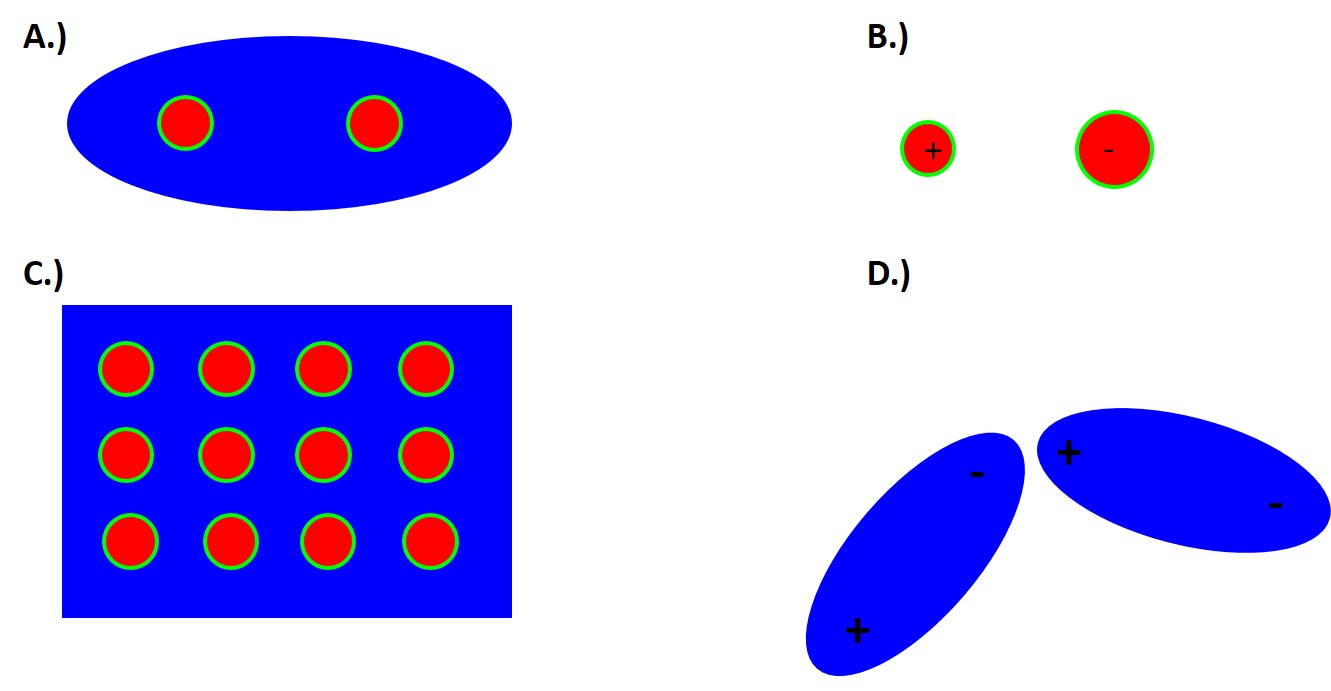
For Van der Waals interactions there is no charge transfer. Instead we have induced electric dipoles or permanent dipoles from weak attractive bonds. With covalent bonds there are valence electrons that are shared between adjacent atoms, which results in a pairing of electrons into localized orbitals and concentrating the negative charge between the positive nuclei.

Now when atoms have a different affinity for electrons, different electronegativities, a net transfer of charge can occur forming positively and negatively charged ions. These ions can form networks of ionic bonds held together by long-range coulombic interactions.

When the electronegativity is similar or the same between atoms the valence electrons are shared equally and the bond is purely covalent.

When the electronegativity is very different the more electronegative atom withdraws nearly all the valence electrons and the bond is purely ionic. Thus electronegativity is how we distinguish between Covalent and Ionic interactions!

Now you might ask what happens in the intermediate case of electronegativity differences. Well then you will have bonds that have both covalent and ionic characteristics. We call these bonds polar covalent and one atom will have a partial positive and negative charge, as in HCl. While there is no universally agreed upon cutoff values in this class we will define an electronegativity difference of 0-0.4 to be non-polar covalent, 0.5-1.7 to be polar covalent, and greater than 1.7 to be ionic.

In the case of metallic bonds, all atoms share their valence electrons and the nuclei form a positively charged array in a sea of delocalized electrons. Van der Waals form between covalently bonded molecules which have net or induced dipoles. These are very short-range force bonds and therefore localized between neighboring molecules. While these bonds are typically very weak and short range these interactions are critical to a number of unique phenomenon, in particular Gecko pads, graphite sheets, water, polymers, and proteins.

1.4.2 Intermolecular Forces/Interactions

As we previously mentioned intermolecular interactions are critical for many soft matter systems and there are several weak intermolecular interactions of interest, which include:

• Hard sphere potentials - the ability of atoms to effectively occupy space and repel at short length scales, quantum mechanical in nature
• Coulombic interactions - electrostatic attraction/repulsion between charged ions
• Lennard-Jones (LJ) potentials - induced dipole interactions between neutral atoms
• Hydrogen bonding - net dipole interactions
• The hydrophobic effect - a largely entropic interaction related to the structuring of water around hydrophobic interfaces.
• Van der Waals force - includes London dispersion force, Debye force, and Keesom force which describe attraction and repulsion due to fluctating polarization between nearby atoms/elements/particle, quantum mechanical in nature. Van der Waals forces decay as d\(^{-6}\).
  

If you are interested in the origin of these interactions there is an excellent book by Israelsachvili I can recommend but the key thing to focus on is that all of these interactions have energies on the order of 1kT, so thermal fluctuations can break these bonds potentially.

1.4.3 Structural Descriptors of Bonding

We also have structural descriptors of bonded materials particularly bond length, bond angles, and the size of atoms or ions. The bond length is simply the distance between two bonds. The distance between a Carbon-Carbon bonds is 1.54\(\AA\) for reference. Bond length can change depending on whether the bond is covalent or ionic. Bond angles} are defined by the relative location of three atoms. In CO\(_{2}\), this molecule is planar so the angle is 180\(^{o}\). For triogonal planar molecules like BF\(_{3}\) the bond angle is 120\(^{o}\). What is the bond angle for our Materials Tetrahedra? It is 109.28\(^{o}\).

The size of an atom is determined by the distance the electron distribution extends from the nucleus. However, this definition is problematic as the type of bonding and bonding in general will change the shape of the electron distribution. So the better value to look for is the covalent, ionic, metallic, and van der Waals radii of the atom. For metals we simply use metallic radii. Covalent radii is one half the covalent bond length. Ionic radii can vary an depends on how many electrons are transferred and the electronegativity difference. The van der Waals radii is the distance of closest approach or approximately the nearest neighbor distance. We will be talking a lot more about the nearest neighbor distances in the next lecture.

The 3D shapes of molecules can be predicted using electron-domain theory} which focuses on the 3D distribution of the outermost electrons about a given atom and how these electrons will pair with other electrons from bonding atoms allen_structure_1999}. This theory distinguishes between bonding and non-bonding domains. The bonding domain is the shared electrons and the non-bonding domain belongs to a particular atom. Nonbonding domains occupies a larger space than the bonding domains. This leads to preferred angles for example for two domains they will be 180\(^{o}\) apart, for 3 it will be 120\(^{o}\), and for 4 it will be 109.28\(^{o}\).

1.4.4 Isomeric States

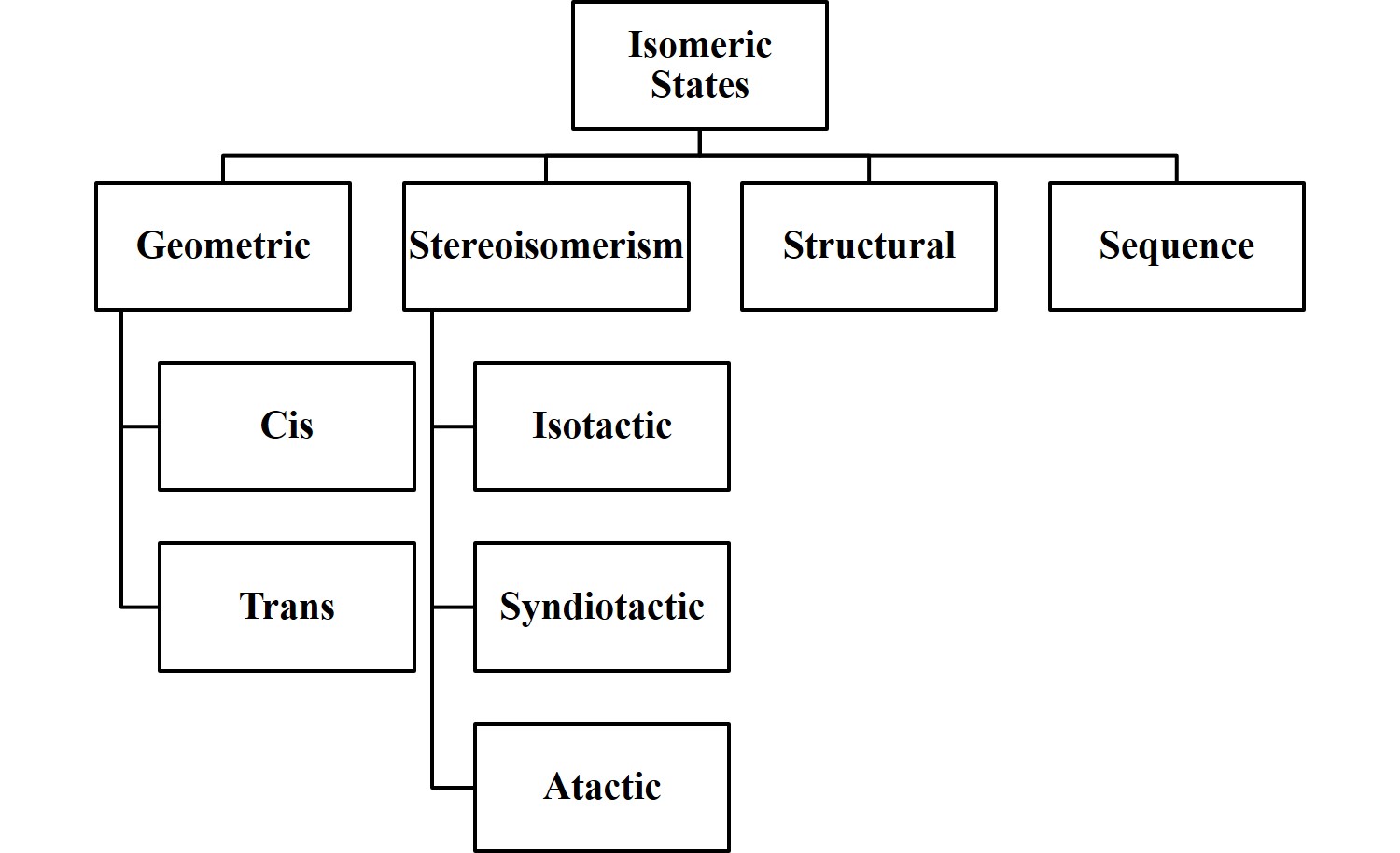
Molecules are typically held together by strong covalent bonds with many conformations available via rotational isomeric states. In other words, conformations are accessible due to the rotation of atoms around these intramolecular bonds. Isomers/Isomeric States are molecules which are compositionally identical but structurally distinct. Conformers/Conformational Isomers are related by rotations around single bonds. Note that at room temperature thermal rotation around a double or triple bond is essentially zero. There are structural isomers, stereoisomers, geometric/configurational, and sequence isomers. Structural isomers occur when certain bonds prohibit rotoconversion of two conformationally distinct states.

ichlorethene is a structural isomer or a geometric isomer. We can see the cis and trans conformations in the figure. Here the double bond prevents rotational so they are structurally distinct. It is a structural isomer not a conformer.

Stereoisomers have an ordered sequence of linked units but the substituents pendant to the main backbone of covalent bonds have different arrangements or tacticity. Specifically they can be atactic, isotactic, or syndiotactic.

Stereoisomers are found in many different types of polymers and we can see an example of atactic, isotactic, and syndiotactic below:

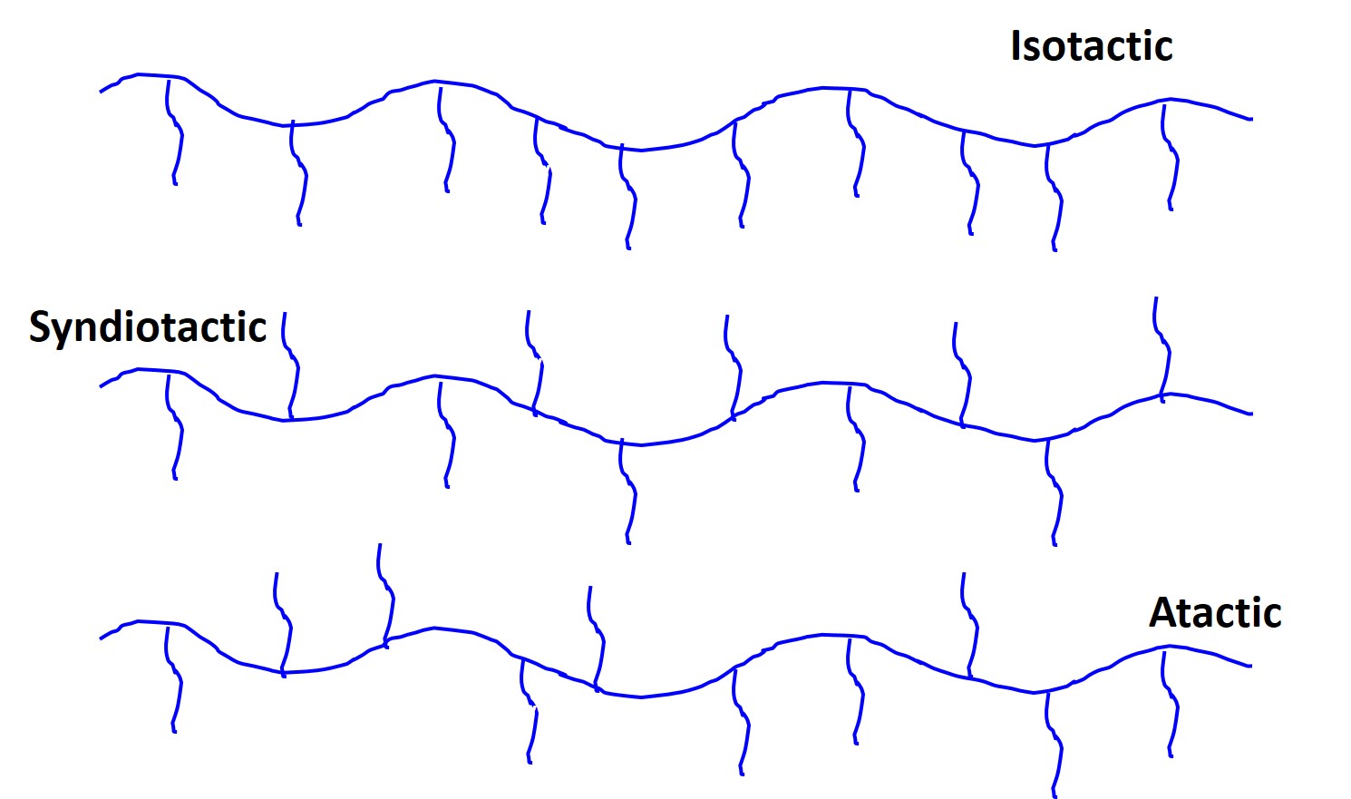
Isotactic stereoisomers will have all the side-chains on the same side. Syndiotactic will have some type of repeated order either top and bottom, or top-top, bottom-bottom, etc. Atactic is completely random.

A geometric/configurational/cis-trans isomer has the same chemical formula but typically the arrangements of the side groups are on different sides of an unsaturated carbon backbone bond. Specifically there will be cis and trans configurations.

Sequence isomers} have many linked units like in a polymer but can have a variable sequence. For example think about block co-polymers which can be designed to be ABABABAB or AAAABBBB.

1.4.5 Coordination Number (CN)

The coordination number (CN) is the number of nearest neighbors (NN). There are a number of coordination shells like the nearest neighbors and the next nearest neighbors (NNN). For liquids and amorphous materials it will typically be an average number of nearest neighbors in a predefined shell of a particular distance or length or Voronoi Tessalation. We will also define and discuss the packing fraction V\(_{v}\) which is the ratio of the total occupied volume to the total volume. For gases this should be very low, almost zero. Fluids or glasses should be about 0.5 and we will see this is much higher for metals and ceramics.