
Chapter 2: Structure: Crystalline, Amorphous, Non-Crystalline, and Liquid Crystal Materials
- Page ID
- 97965

\( \newcommand{\vecs}[1]{\overset { \scriptstyle \rightharpoonup} {\mathbf{#1}} } \)
\( \newcommand{\vecd}[1]{\overset{-\!-\!\rightharpoonup}{\vphantom{a}\smash {#1}}} \)
\( \newcommand{\dsum}{\displaystyle\sum\limits} \)
\( \newcommand{\dint}{\displaystyle\int\limits} \)
\( \newcommand{\dlim}{\displaystyle\lim\limits} \)
\( \newcommand{\id}{\mathrm{id}}\) \( \newcommand{\Span}{\mathrm{span}}\)
( \newcommand{\kernel}{\mathrm{null}\,}\) \( \newcommand{\range}{\mathrm{range}\,}\)
\( \newcommand{\RealPart}{\mathrm{Re}}\) \( \newcommand{\ImaginaryPart}{\mathrm{Im}}\)
\( \newcommand{\Argument}{\mathrm{Arg}}\) \( \newcommand{\norm}[1]{\| #1 \|}\)
\( \newcommand{\inner}[2]{\langle #1, #2 \rangle}\)
\( \newcommand{\Span}{\mathrm{span}}\)
\( \newcommand{\id}{\mathrm{id}}\)
\( \newcommand{\Span}{\mathrm{span}}\)
\( \newcommand{\kernel}{\mathrm{null}\,}\)
\( \newcommand{\range}{\mathrm{range}\,}\)
\( \newcommand{\RealPart}{\mathrm{Re}}\)
\( \newcommand{\ImaginaryPart}{\mathrm{Im}}\)
\( \newcommand{\Argument}{\mathrm{Arg}}\)
\( \newcommand{\norm}[1]{\| #1 \|}\)
\( \newcommand{\inner}[2]{\langle #1, #2 \rangle}\)
\( \newcommand{\Span}{\mathrm{span}}\) \( \newcommand{\AA}{\unicode[.8,0]{x212B}}\)
\( \newcommand{\vectorA}[1]{\vec{#1}} % arrow\)
\( \newcommand{\vectorAt}[1]{\vec{\text{#1}}} % arrow\)
\( \newcommand{\vectorB}[1]{\overset { \scriptstyle \rightharpoonup} {\mathbf{#1}} } \)
\( \newcommand{\vectorC}[1]{\textbf{#1}} \)
\( \newcommand{\vectorD}[1]{\overrightarrow{#1}} \)
\( \newcommand{\vectorDt}[1]{\overrightarrow{\text{#1}}} \)
\( \newcommand{\vectE}[1]{\overset{-\!-\!\rightharpoonup}{\vphantom{a}\smash{\mathbf {#1}}}} \)
\( \newcommand{\vecs}[1]{\overset { \scriptstyle \rightharpoonup} {\mathbf{#1}} } \)
\(\newcommand{\longvect}{\overrightarrow}\)
\( \newcommand{\vecd}[1]{\overset{-\!-\!\rightharpoonup}{\vphantom{a}\smash {#1}}} \)
\(\newcommand{\avec}{\mathbf a}\) \(\newcommand{\bvec}{\mathbf b}\) \(\newcommand{\cvec}{\mathbf c}\) \(\newcommand{\dvec}{\mathbf d}\) \(\newcommand{\dtil}{\widetilde{\mathbf d}}\) \(\newcommand{\evec}{\mathbf e}\) \(\newcommand{\fvec}{\mathbf f}\) \(\newcommand{\nvec}{\mathbf n}\) \(\newcommand{\pvec}{\mathbf p}\) \(\newcommand{\qvec}{\mathbf q}\) \(\newcommand{\svec}{\mathbf s}\) \(\newcommand{\tvec}{\mathbf t}\) \(\newcommand{\uvec}{\mathbf u}\) \(\newcommand{\vvec}{\mathbf v}\) \(\newcommand{\wvec}{\mathbf w}\) \(\newcommand{\xvec}{\mathbf x}\) \(\newcommand{\yvec}{\mathbf y}\) \(\newcommand{\zvec}{\mathbf z}\) \(\newcommand{\rvec}{\mathbf r}\) \(\newcommand{\mvec}{\mathbf m}\) \(\newcommand{\zerovec}{\mathbf 0}\) \(\newcommand{\onevec}{\mathbf 1}\) \(\newcommand{\real}{\mathbb R}\) \(\newcommand{\twovec}[2]{\left[\begin{array}{r}#1 \\ #2 \end{array}\right]}\) \(\newcommand{\ctwovec}[2]{\left[\begin{array}{c}#1 \\ #2 \end{array}\right]}\) \(\newcommand{\threevec}[3]{\left[\begin{array}{r}#1 \\ #2 \\ #3 \end{array}\right]}\) \(\newcommand{\cthreevec}[3]{\left[\begin{array}{c}#1 \\ #2 \\ #3 \end{array}\right]}\) \(\newcommand{\fourvec}[4]{\left[\begin{array}{r}#1 \\ #2 \\ #3 \\ #4 \end{array}\right]}\) \(\newcommand{\cfourvec}[4]{\left[\begin{array}{c}#1 \\ #2 \\ #3 \\ #4 \end{array}\right]}\) \(\newcommand{\fivevec}[5]{\left[\begin{array}{r}#1 \\ #2 \\ #3 \\ #4 \\ #5 \\ \end{array}\right]}\) \(\newcommand{\cfivevec}[5]{\left[\begin{array}{c}#1 \\ #2 \\ #3 \\ #4 \\ #5 \\ \end{array}\right]}\) \(\newcommand{\mattwo}[4]{\left[\begin{array}{rr}#1 \amp #2 \\ #3 \amp #4 \\ \end{array}\right]}\) \(\newcommand{\laspan}[1]{\text{Span}\{#1\}}\) \(\newcommand{\bcal}{\cal B}\) \(\newcommand{\ccal}{\cal C}\) \(\newcommand{\scal}{\cal S}\) \(\newcommand{\wcal}{\cal W}\) \(\newcommand{\ecal}{\cal E}\) \(\newcommand{\coords}[2]{\left\{#1\right\}_{#2}}\) \(\newcommand{\gray}[1]{\color{gray}{#1}}\) \(\newcommand{\lgray}[1]{\color{lightgray}{#1}}\) \(\newcommand{\rank}{\operatorname{rank}}\) \(\newcommand{\row}{\text{Row}}\) \(\newcommand{\col}{\text{Col}}\) \(\renewcommand{\row}{\text{Row}}\) \(\newcommand{\nul}{\text{Nul}}\) \(\newcommand{\var}{\text{Var}}\) \(\newcommand{\corr}{\text{corr}}\) \(\newcommand{\len}[1]{\left|#1\right|}\) \(\newcommand{\bbar}{\overline{\bvec}}\) \(\newcommand{\bhat}{\widehat{\bvec}}\) \(\newcommand{\bperp}{\bvec^\perp}\) \(\newcommand{\xhat}{\widehat{\xvec}}\) \(\newcommand{\vhat}{\widehat{\vvec}}\) \(\newcommand{\uhat}{\widehat{\uvec}}\) \(\newcommand{\what}{\widehat{\wvec}}\) \(\newcommand{\Sighat}{\widehat{\Sigma}}\) \(\newcommand{\lt}{<}\) \(\newcommand{\gt}{>}\) \(\newcommand{\amp}{&}\) \(\definecolor{fillinmathshade}{gray}{0.9}\)2.1 Crystal Structures
We will eventually talk about crystalline materials, amorphous materials, liquid crystals, short range order, long range order, etc. But to start we are going to deal with the most ideal case of perfect crystalline materials.
Do we ever have a perfect crystal? No! Why? Well maybe at 0K but even then still probably not. There are always defects in materials but let’s start with the simple case where we assume everything is perfect.
A crystal structure is a periodic array of atoms that repeats over large distances. There is long-range periodic order both long range translational and orientational order in addition to short range order. So before we start to run off and analyze crystal structures we have to first start off with a primitive lattice, lattice constants, interaxial angles, symmetries, point groups, Bravais lattices....
I have recorded a series of videos to supplement this text which can be found in the playlist here:
2.2 Lattice, Primitive Unit Cell, Basis Vectors, Lattice Constants
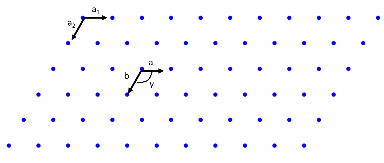
A lattice is a periodic array of points (atoms) in 1,2 or 3D. Those points are lattice points. Let’s start with the 2D case. A 2D lattice can be described by a primitive or unit cell which in turn is described by two lattice constants (a,b), two basis vectors (a\(_1\) and a\(_2\)) an interaxial angle \(\gamma\). Once we have defined this we can pick any point in our 2D lattice as an origin and we can describe any point in our lattice with the previous values. That is the beauty of crystallography!
Now when we pick our basis vectors we pick the shortest lattice translation as a\(_1\) and the second to shortest translation is a\(_2\). The lattice constants are the just given by a \(= |a_1|\) and b = \(= |a_2|\) The interaxial angle γ is then simply defined. This also defines our primitive cell which will only contain a single lattice point. Let’s do a couple of examples looking at the parallelogram cell below:
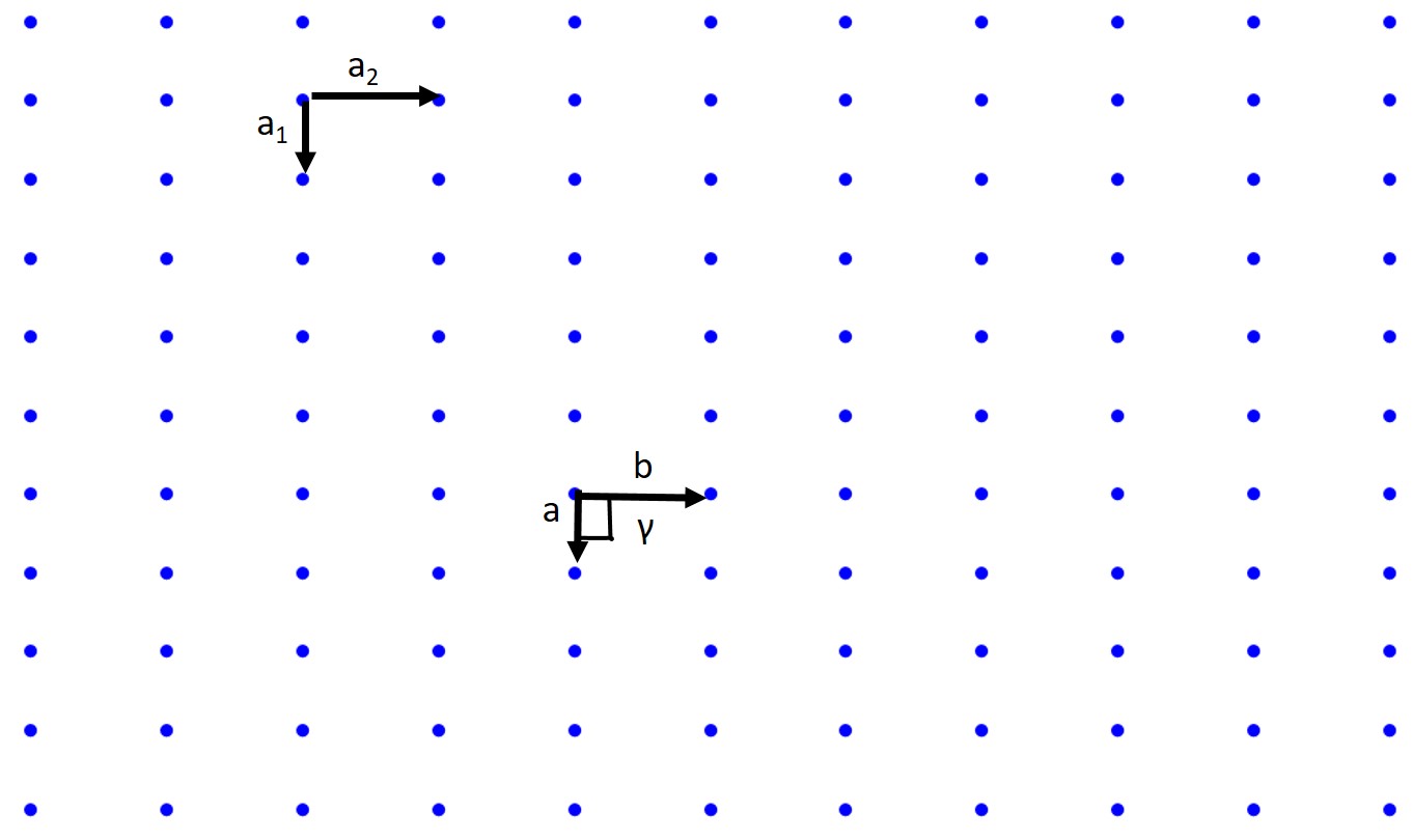
How about a Rectangular lattice?
Associated with crystallography is a myriad of symmetry operations and we have actually just dealt with translational symmetry just now. There are also reflection or mirror symmetry, glide symmetry, rotational symmetry, etc. These topics are all important but we are not a crystallography class so we will not be covering this in detail but you should know these concepts exist. There are also 230 space groups, 32 crystallographic point groups, 14 Bravais lattices (we will discuss these), and 6 crystal systems (will discuss these as well).
2.3 Crystal Systems: Simple Cubic, BCC, FCC, HCP
We are going to focus on the 6 crystal systems: triclinic, monoclinic, orthorhombic, tetragonal, hexagonal, and cubic and how to describe the unit cell, the primitive lattice vectors, and interaxial angles.
2.3.1 Crystallographic Directions:
When discussing crystals we will also have to specify crystallographic directions and planes. In order to refer to specific crystallographic planes or direction we need a labeling system to index these directions or planes. Luckily such an index has already been developed, Miller indices. A crystallographic direction is a vector denoted by [uvw]. u,v, and w are integers which correspond to the reduced projections along the x,y, and z axes, respectively. Note we will always use [] for vectors. Let’s do a couple of examples.
Let start simple and draw the [100] direction.
To draw the direction of a vector it is pretty straight forward. Pick an origin for the vector tail (side without arrow) then pick the ending point for the vector (arrow) and subtract the arrow point from the tail point and the resultant vector must coincide with the direction that you are trying to draw. Typically try to pick the origin as your origin.
How about the [111] direction?
What about [100]?
Little more complicated what about [110]?
What about drawing [222]?
Now a little more complicated what is the vector I am drawing below?
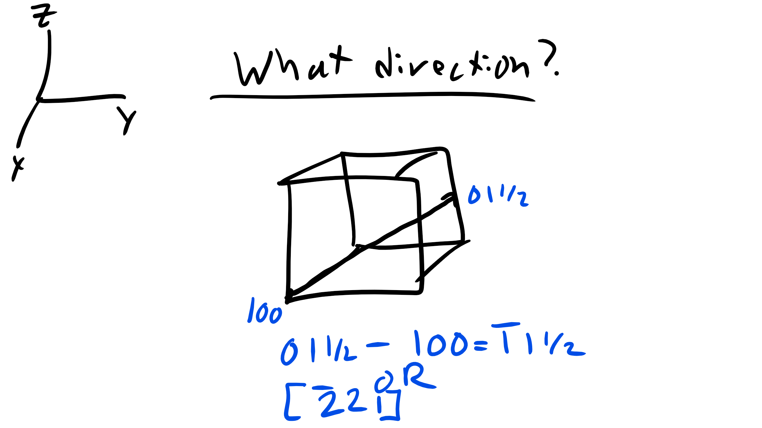
Now for a number of crystal structures there are several nonparallel directions with different indices that are crystallographically equivalent. This means that the spacing and number of atoms along each direction is the same! In cubic crystals [100],[100],[010],[010],[001], and [001] are all crystallographically equivalent so we group them in a family which is denoted by angled brackets < 100>.
2.3.2 Crystallographic Planes:
Now for crystallographic planes we utilize the Miller indicies (hkl) which corresponds to the x,y, and z axes respectively. Notice again that we use () for planes and [] for directions. <> is for family of directions. We will denote families of planes in {}.
Now the question becomes how do we draw planes. Well we first must determine if the intercepts. The intercepts will be the inverse of the Miller indices. Let’s take a look at a relatively straightforward example of the (111).
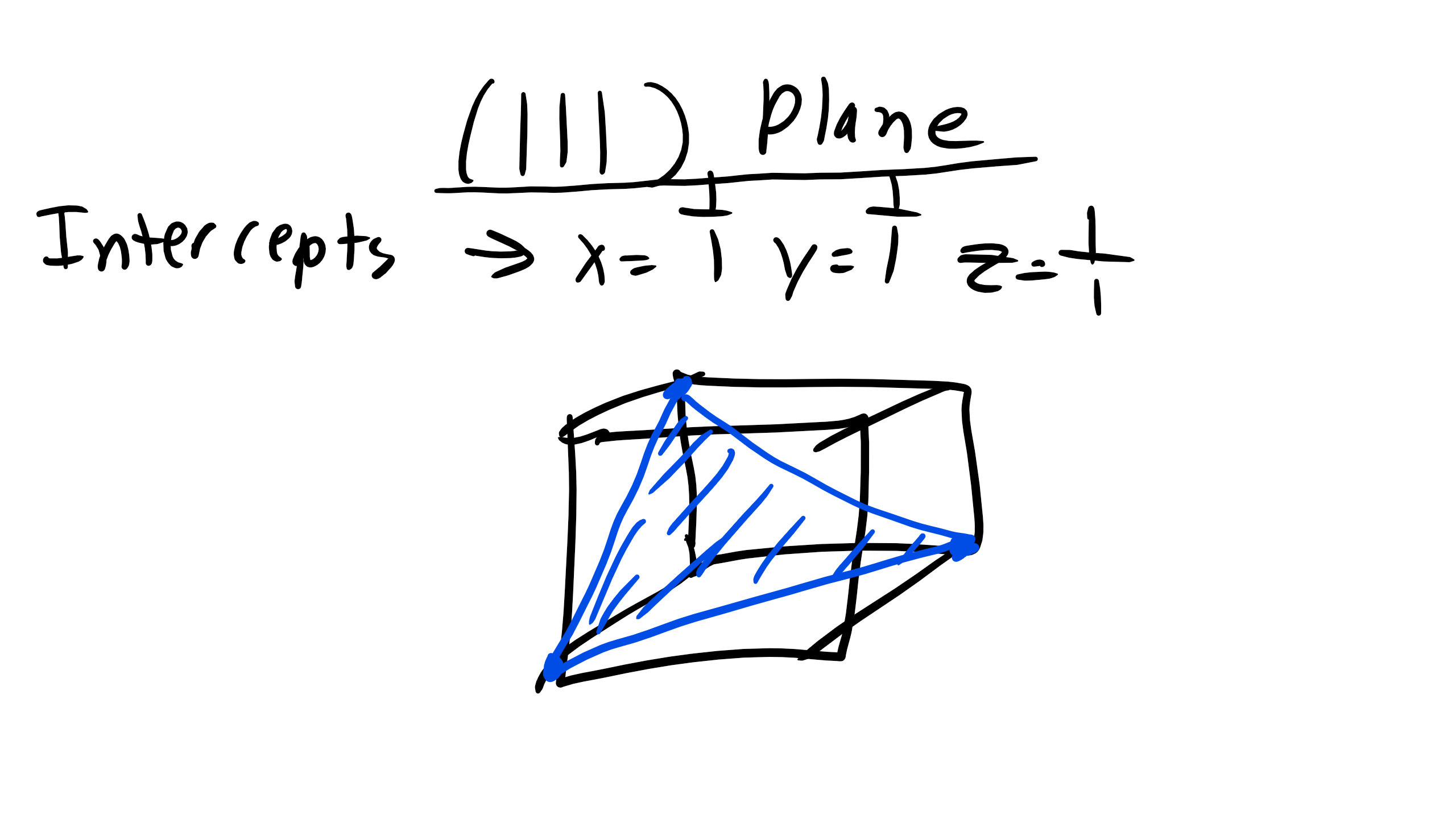
Figure \(\PageIndex{4}\): (111) Crystallographic Plane
Now what happens in the case of (110) for example. Well if you run into this problem an inverse that gives you an infinite number means that the plane will not intersect that coordinate axes and will instead be parallel to that axis. So the plane should look like this:
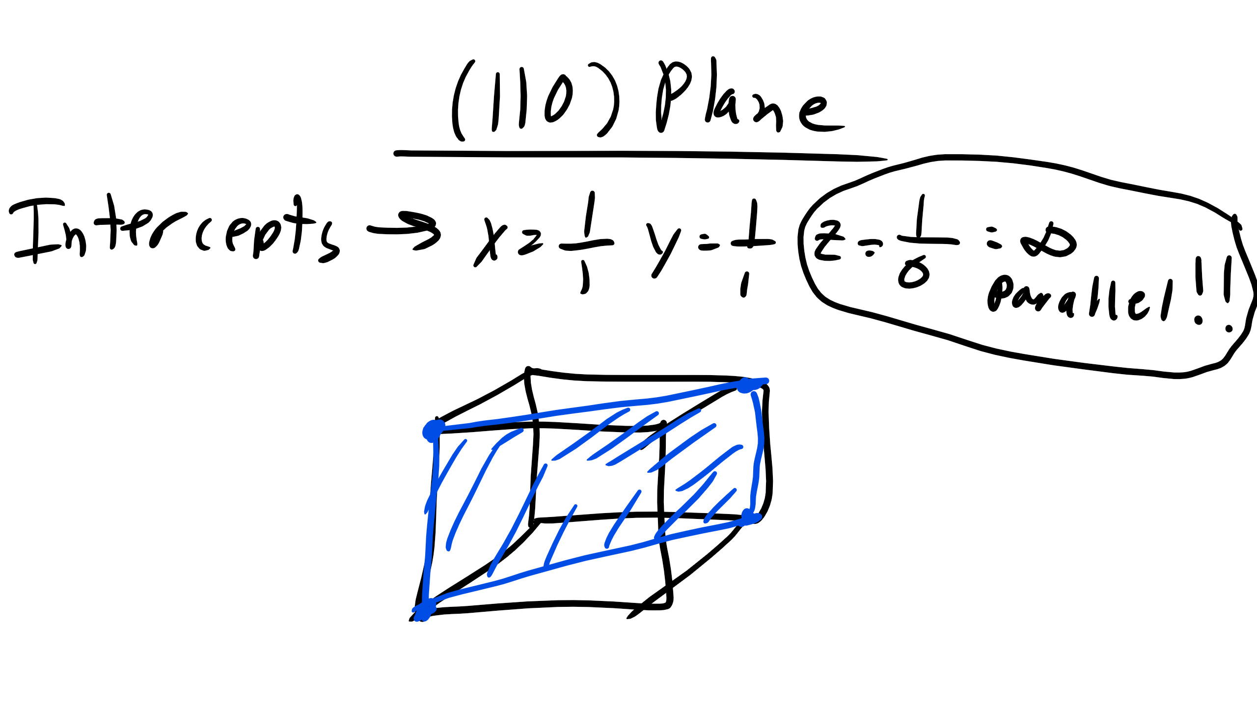
Figure \(\PageIndex{5}\): (110) Crystallographic Plane.
How about another tricky problem like below when we have the plane passing through our origin?
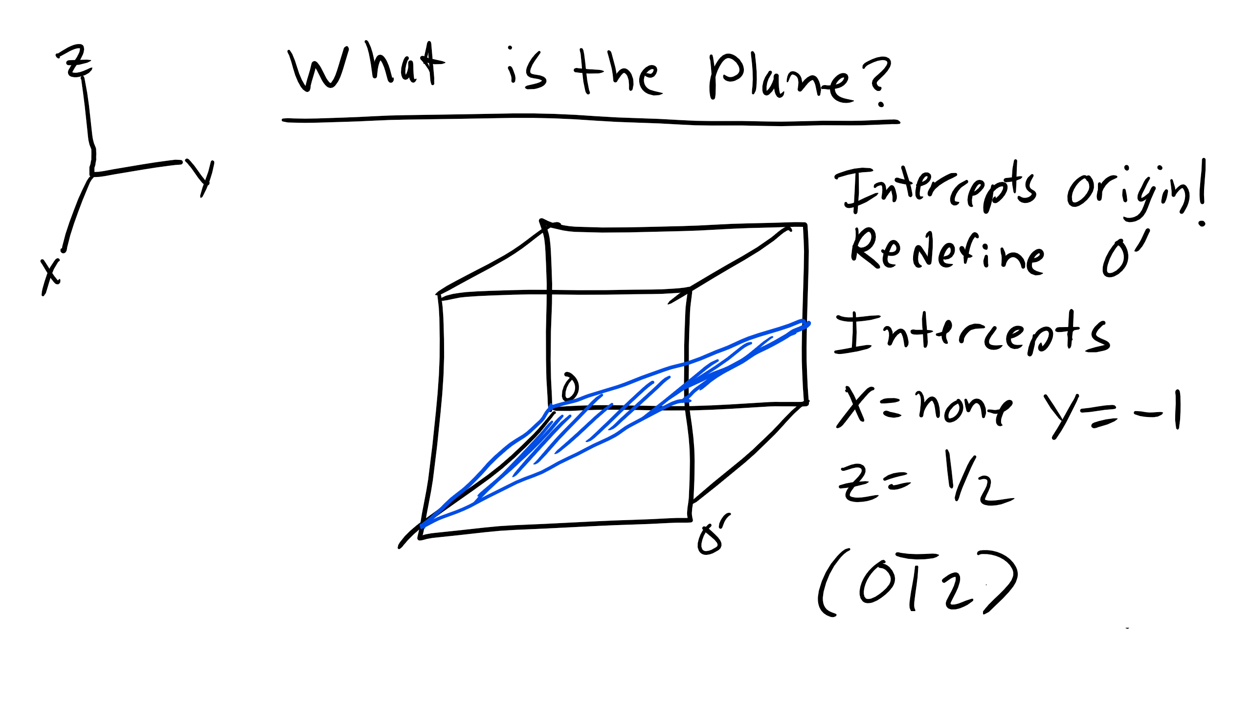
Here all the axes appear to be intersected, there are no parallel planes. True but this is actually misleading. When you have a plane that intersects the origin you need to choose a different origin and go through the same procedure to determine where the plane intercepts and then we can find the Miller indices of the plane.
The plane intercepts are again the inverse of the Miller indices and families of planes are denote in curly brackets hkl.
Here is a nice demonstration to visualize the Crystallographic Planes:
https://demonstrations.wolfram.com/PlanarDensityOfCrystallographicPlanesInSCBCCAndFCCCrystals/
2.3.3 Anisotropy
Now it’s important to mention that we have been assuming until now that material properties are the same in every direction however this is not actually the case. Often many materials are anisotropic, meaning that some materials properties (mechanical, optical, kinetic, etc.) are different depending on the crystallographic direction you are investigating. For example titanium exhibits a larger modulus along the z-axis in the HCP structure than in the basal plane. This presents a significant problem when trying to superplastically form very thin foil made of titanium. A similar issue arises with magnetic properties of HCP materials as well. You should always remember as well that materials are not one perfect single crystal instead they are made of multiple crystalline grains, i.e. they are polycrystalline.
2.4 Simple Cubic
So let’s start simple with the simple cubic to begin. So the simple cubic (SC) is also sometimes called primitive cubic and it is the crystal structure for Oxygen, Fluorine, etc. As you can see below it is described by the primitive lattice vectors \(a_1\), \(a_2\), and \(a_3\) and interaxial angles \(\alpha\) (angle between \(a_2\) and \(a_3\)), \(\beta\) (angle between \(a_1\) and \(a_3\)), and \(\gamma\) (angle between \(a_1\) and \(a_2\)).
Notice the figure on the right is how the structure actually looks with the atoms touching. Here \(\alpha = \beta = \gamma = 90^o\). For simple cubic structures \(a_1 = a[100], a_2 = [010], and a_3 = [001]\). Right now I want to point that this is going to be the vector notation we use to signify a direction in a crystal lattice, more on this a bit later. And for this case the lattice constants are all equal a = b = c = a = 2R where R is the atomic radius of our element.
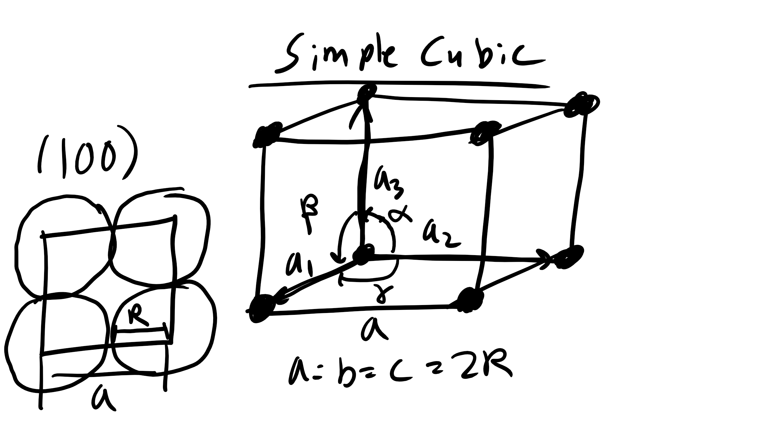
Figure \(\PageIndex{7}\): Simple cubic unit cell.
How many atoms are contained in our simple cubic cell?
Well it is simply 1 because the all the corner atoms are shared by 8 other unit cells so
How many nearest neighbors (NN) does each atom have?
6.
How many second nearest neighbors?
12.
What is the NN distance?
2R
What about the NNN distance?
2R\(\sqrt{2}\)
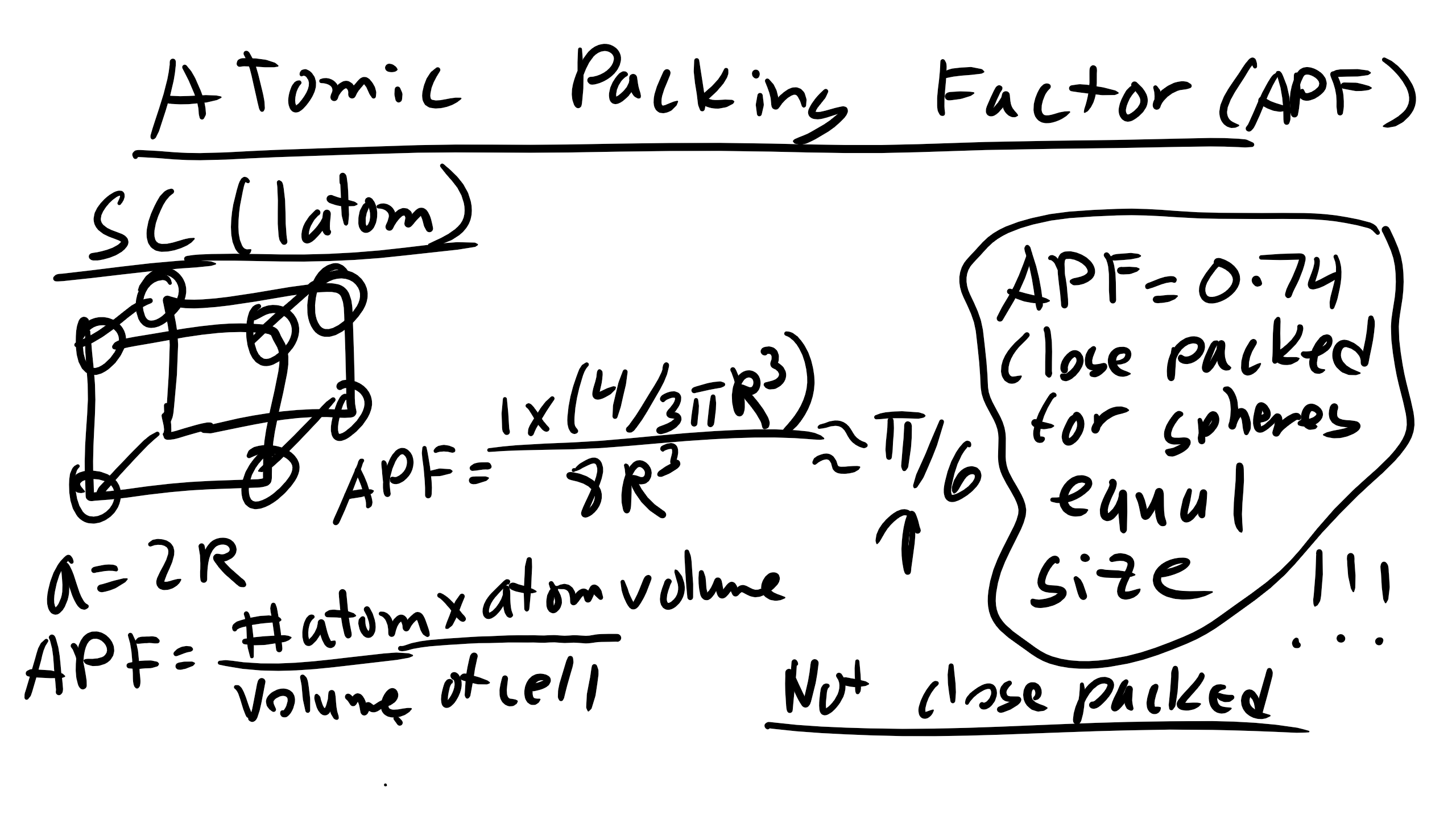
What about the atomic packing factor?
To calculate this we must calculate the volume of atoms in a unit cell by the total unit cell volume. Well for simple cubic we know that the volume of our conventional unit cell is \(a^3\). Additionally with the simple cubic lattice we only have 1 atom so that volume is simply \(\frac{4}{3} \pi R^{3}\) so plugging and chugging we get
2.5 Body Center Cubic (BCC)
Let’s look at a little more complicated cubic structure, body centered cubic (BCC). BCC is the structure for Li, Fe, V, Mo.
BCC is described by the primitive \(a_{1} = \frac{a}{2}[1 \overline{1} 1], a_{2} = \frac{a}{2}[1 1 \overline{1}], and a_{3} = \frac{a}{2}[\overline{1} 1 1] and \alpha = \beta = \gamma = 90^{o}\).
What is a now? Is it still 2R? No it is not!!
Now \(a = \frac{4R}{\sqrt{3}}\) where again R is the atomic radius which can be solved using a little bit of geometry.
How many atoms in a BCC conventional unit cell?
It is 2 atoms this time one in the interior and then 8 shared atoms so 2 total.
How many NN?
8.
How many NNN?
6.
What is the NN distance?
2R.
What about the second nearest neighbor distance?
It is simply \(\frac{4R}{\sqrt{3}}\).
What about the atomic packing factor?
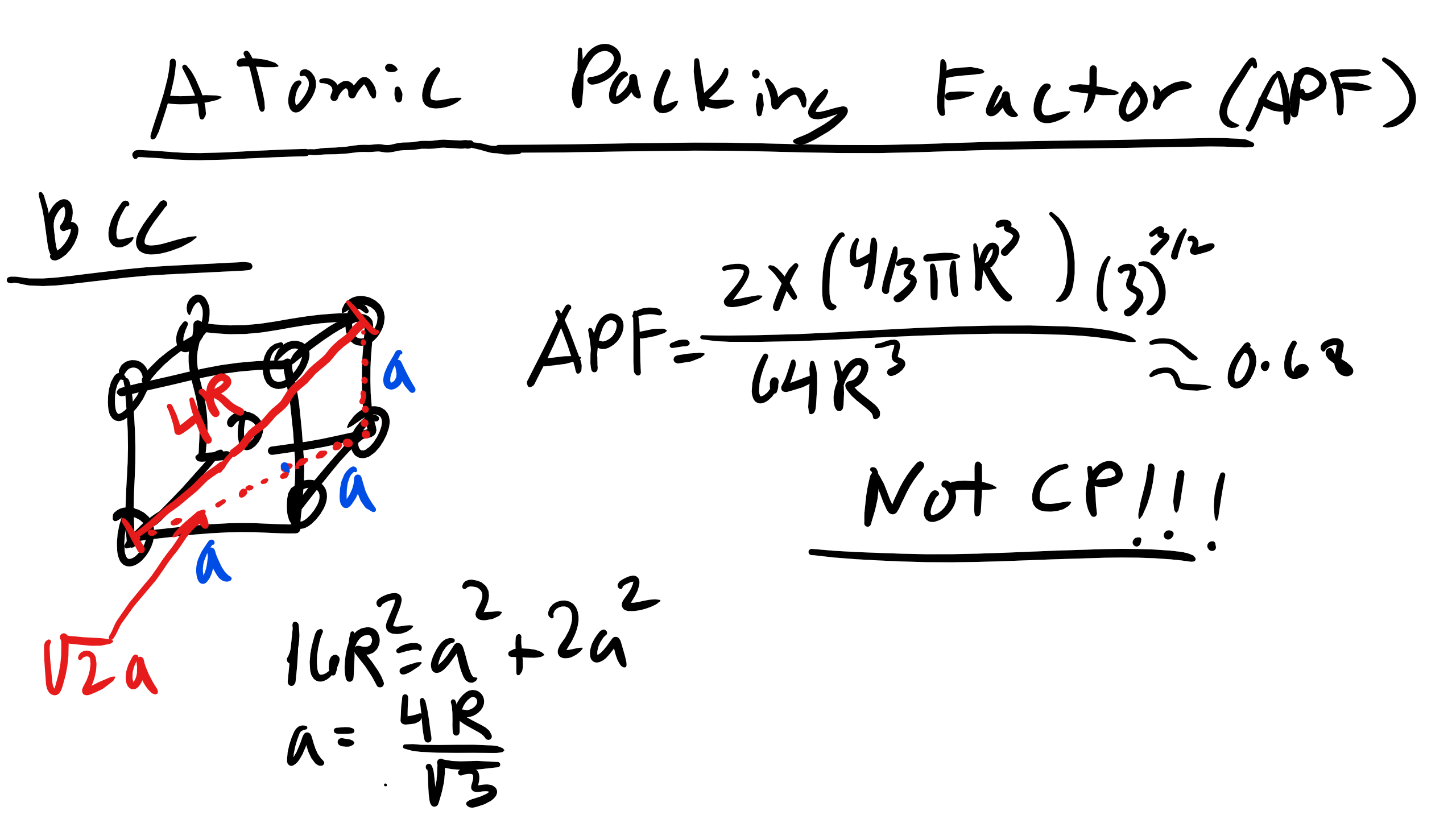
It is 0.68.
How did we get that? Well again how many atoms in a conventional BCC unit cell? 2 atoms.
We also know the volume of our unit cell know since we found a. Double check!
2.6 Face Centered Cubic (FCC)
Next is face centered cubic (FCC). FCC is the structure for Ni, Cu, Ca and it is described by the primitive lattice vectors \(a_{1} = \frac{a}{2}[0 1 1], a_{1} = \frac{a}{2}[1 0 1], and a_{2} = \frac{a}{2}[1 1 0] and \alpha = \beta = \gamma = 90^{o}\). Here \(a = 2 \sqrt{2}R\) where again R is the atomic radius. Remember that the primitive unit cell will have only a single atom but a conventional cell may not.
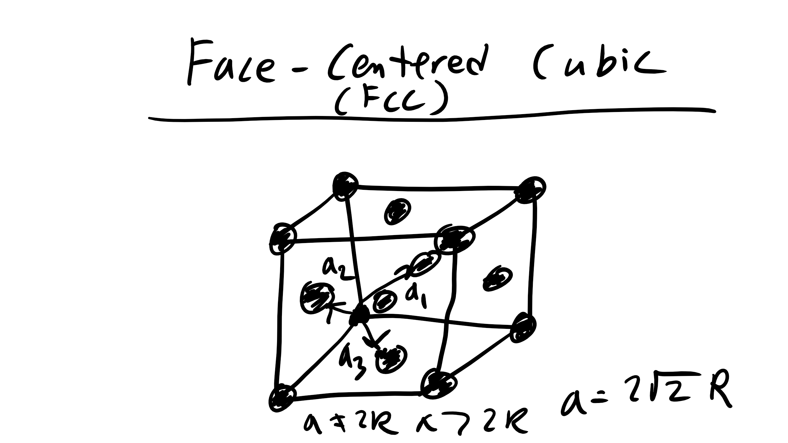
Remember that the primitive unit cell will have only a single atom but a conventional cell may not.
How many atoms in a FCC unit cell?
It is 4 atoms this time 8 share on the edges and 6 shared on the faces.
How many NN?
12.
How many NNN?
6.
What is the NN distance?
2R
What about the second nearest neighbor distance?
2R\(\sqrt{2}\)
What about the atomic packing factor?
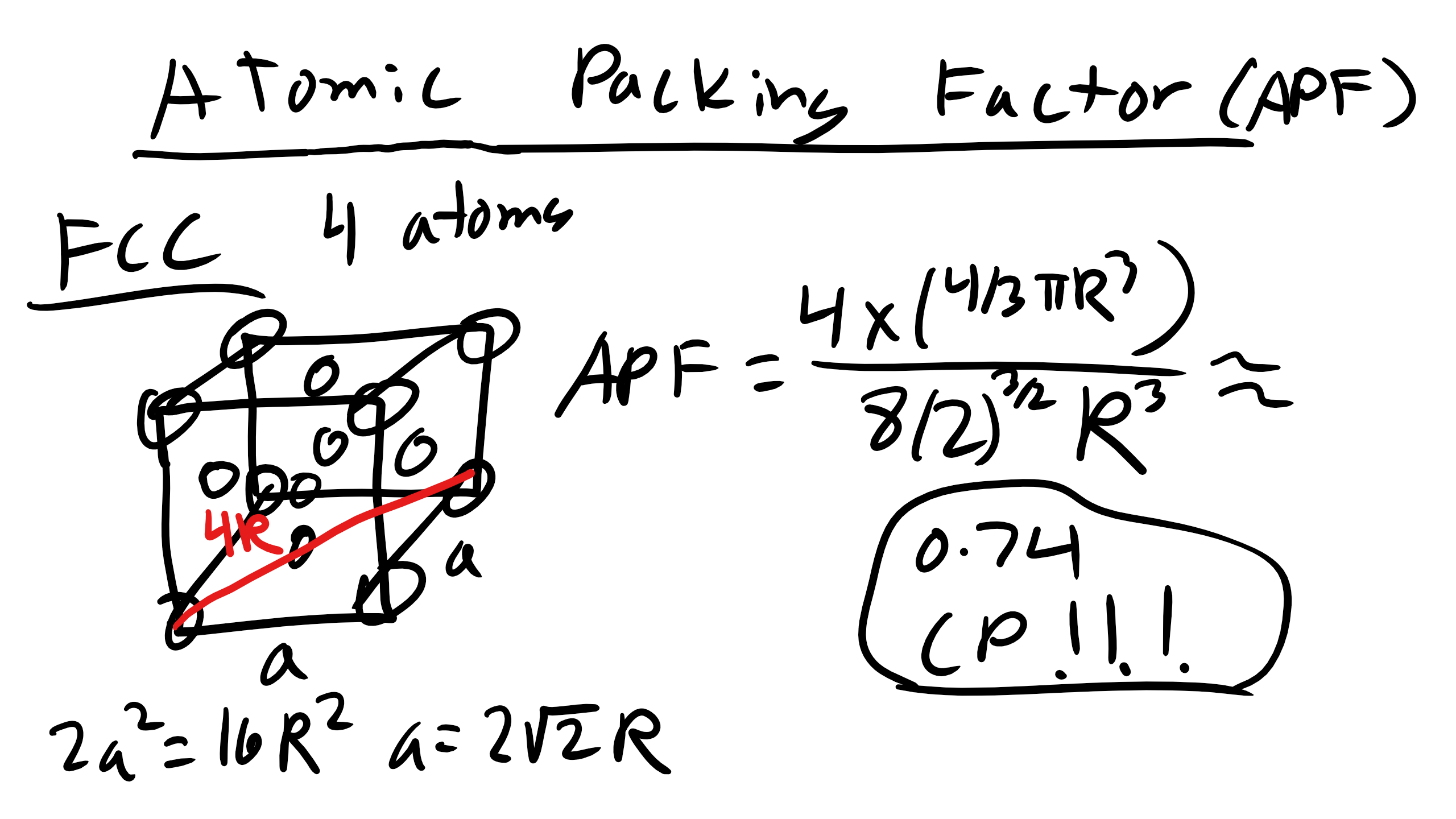
What about the atomic packing factor?
It is 0.74.
This is the maximum possible packing factor for spheres having all the same diameter.
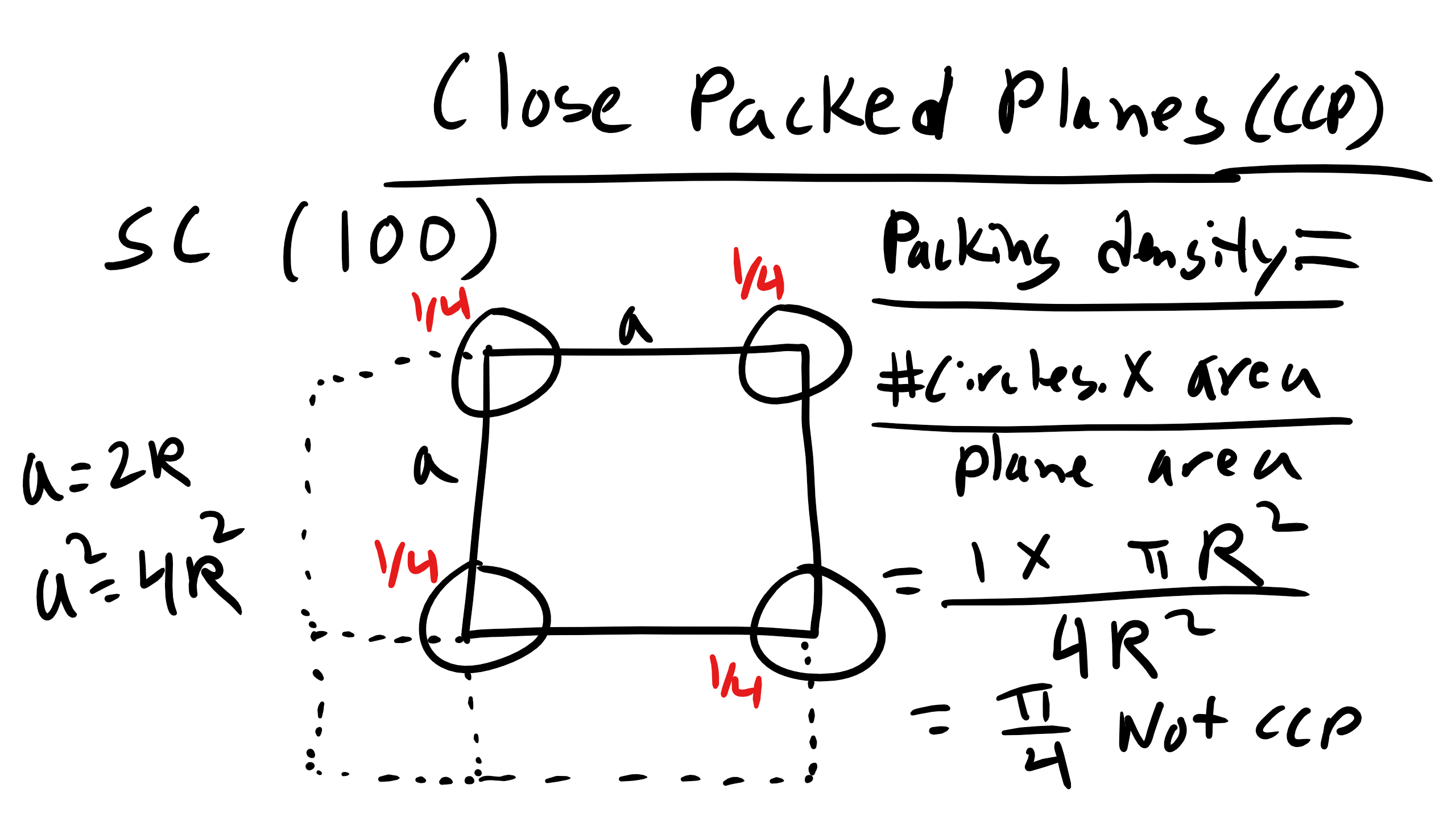
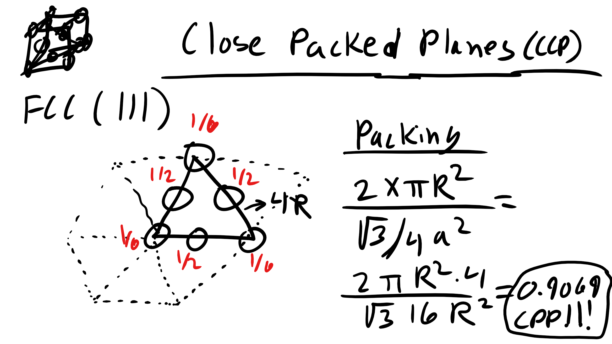
A close-packed plane is defined as a plane with an packing density of approximately
0.9069.
What is the packing density for the (100) plane in SC?
What about the (110) plane in BCC?
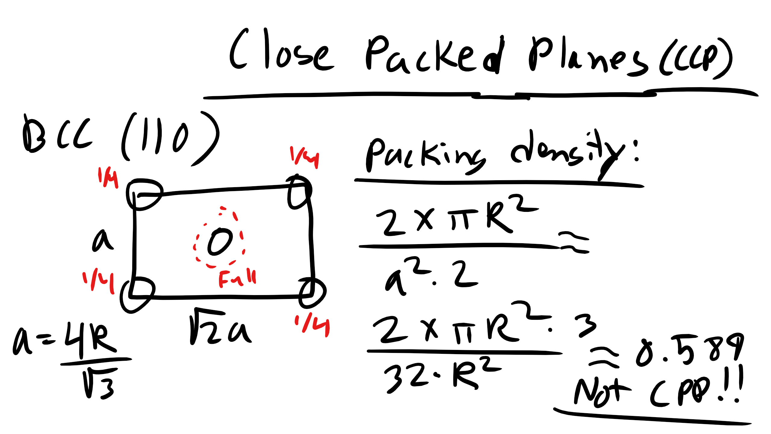
Figure \(\PageIndex{13}\): Planar Density of (110) in BCC.
What about the (111) plane in FCC?
Note that only close packed structures can have close packed planes but often we will be concerned (especially when we talk about diffusion, defects, and mechanics) about the closest packed plane in a crystal and that doesn’t have to have a density of 0.9069.
What are the close packed planes and directions for BCC, FCC, and HCP?
Now when materials have more than one crystals structure they are polymorphic. In elemental solids this phenomenon is called allotropy. You have encountered a number of polymorphic materials, some of you may be holding one in your hand. At least in the old days before tablets. It’s carbon! Carbon can adopt a number of different structures i.e. diamond, graphite, fullerines, graphene.) Iron (BCC and FCC) and Titanium (HCP and BCC) are also polymorphs. We will also investigate lead titanate, a polymorph, in our XRD lab.
2.7 Structure of Non-Crystalline Materials:
2.7.1 Polymers, Liquids, Glasses, Gas, and Liquid Crystals:
Now so far we have focused only on crystalline materials primarily because they are the simplest materials to characterize in terms of structure. However there are many more materials that do not adopt a simple crystalline structure with short range, long range translational, and long range orientational order. Specifically, polymers, liquids, gases, liquid crystals, glasses, and many others.
With crystalline materials we were able to translate a unit cell to essentially infinity. That is because we had both short range order, long range translational order, and long range orientational order. In polymers, glasses, and liquid crystals typically we will only have short range order (SRO) and perhaps some degree of long range order either translational or orientational but typically not both and not to the periodic nature of crystalline materials. So how are we going to talk about structure in these non-crystalline materials which are often incorrectly called disordered materials. Well we are going to use a dimensionless pair distribution function (PDF) or the radial distribution function (RDF), this is also called the pair correlation function as well I know very confusing, which is our key descriptor for quantifying the SRO present in a material.
The PDF or RDF, g(r), is:
\begin{equation}
g(r) = \frac{1}{<\rho>}\frac{dn(r, r+dr)}{dv(r, r+dr)}
\end{equation}
where \(\rho\) is the average particle number density, dn is the number of particles counted in a small spherical shell sampling volume element of size dv at each distance r from a particle chosen as the origin. The number of particles in each shell is counted at each subsequent dr shell. This is shown schematically below
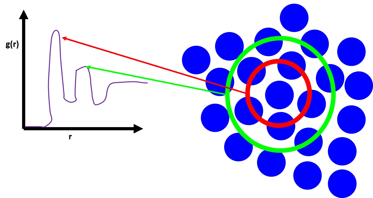
To get a smooth curve you want to pick a very small dr so that is much smaller than the radius of the particle and we must average this over multiple particles chosen as the origin. For perfect crystals we will see the PDF exhibit a series of sharp and discrete peaks at precise values of interatomic spacings which will correspond to the particular crystal structure. Now for liquids you will see a large peak and then some much smaller peaks. This first peak corresponds to your number of nearest neighbors which can be derived by the following equation:
\begin{equation}
<NN> = <\rho> \int_{peak} g(r) 4 \pi r^2 dr
\end{equation}