
Chapter 3: Probability Distributions and the Gaussian
- Page ID
- 99694
\( \newcommand{\vecs}[1]{\overset { \scriptstyle \rightharpoonup} {\mathbf{#1}} } \)
\( \newcommand{\vecd}[1]{\overset{-\!-\!\rightharpoonup}{\vphantom{a}\smash {#1}}} \)
\( \newcommand{\dsum}{\displaystyle\sum\limits} \)
\( \newcommand{\dint}{\displaystyle\int\limits} \)
\( \newcommand{\dlim}{\displaystyle\lim\limits} \)
\( \newcommand{\id}{\mathrm{id}}\) \( \newcommand{\Span}{\mathrm{span}}\)
( \newcommand{\kernel}{\mathrm{null}\,}\) \( \newcommand{\range}{\mathrm{range}\,}\)
\( \newcommand{\RealPart}{\mathrm{Re}}\) \( \newcommand{\ImaginaryPart}{\mathrm{Im}}\)
\( \newcommand{\Argument}{\mathrm{Arg}}\) \( \newcommand{\norm}[1]{\| #1 \|}\)
\( \newcommand{\inner}[2]{\langle #1, #2 \rangle}\)
\( \newcommand{\Span}{\mathrm{span}}\)
\( \newcommand{\id}{\mathrm{id}}\)
\( \newcommand{\Span}{\mathrm{span}}\)
\( \newcommand{\kernel}{\mathrm{null}\,}\)
\( \newcommand{\range}{\mathrm{range}\,}\)
\( \newcommand{\RealPart}{\mathrm{Re}}\)
\( \newcommand{\ImaginaryPart}{\mathrm{Im}}\)
\( \newcommand{\Argument}{\mathrm{Arg}}\)
\( \newcommand{\norm}[1]{\| #1 \|}\)
\( \newcommand{\inner}[2]{\langle #1, #2 \rangle}\)
\( \newcommand{\Span}{\mathrm{span}}\) \( \newcommand{\AA}{\unicode[.8,0]{x212B}}\)
\( \newcommand{\vectorA}[1]{\vec{#1}} % arrow\)
\( \newcommand{\vectorAt}[1]{\vec{\text{#1}}} % arrow\)
\( \newcommand{\vectorB}[1]{\overset { \scriptstyle \rightharpoonup} {\mathbf{#1}} } \)
\( \newcommand{\vectorC}[1]{\textbf{#1}} \)
\( \newcommand{\vectorD}[1]{\overrightarrow{#1}} \)
\( \newcommand{\vectorDt}[1]{\overrightarrow{\text{#1}}} \)
\( \newcommand{\vectE}[1]{\overset{-\!-\!\rightharpoonup}{\vphantom{a}\smash{\mathbf {#1}}}} \)
\( \newcommand{\vecs}[1]{\overset { \scriptstyle \rightharpoonup} {\mathbf{#1}} } \)
\(\newcommand{\longvect}{\overrightarrow}\)
\( \newcommand{\vecd}[1]{\overset{-\!-\!\rightharpoonup}{\vphantom{a}\smash {#1}}} \)
\(\newcommand{\avec}{\mathbf a}\) \(\newcommand{\bvec}{\mathbf b}\) \(\newcommand{\cvec}{\mathbf c}\) \(\newcommand{\dvec}{\mathbf d}\) \(\newcommand{\dtil}{\widetilde{\mathbf d}}\) \(\newcommand{\evec}{\mathbf e}\) \(\newcommand{\fvec}{\mathbf f}\) \(\newcommand{\nvec}{\mathbf n}\) \(\newcommand{\pvec}{\mathbf p}\) \(\newcommand{\qvec}{\mathbf q}\) \(\newcommand{\svec}{\mathbf s}\) \(\newcommand{\tvec}{\mathbf t}\) \(\newcommand{\uvec}{\mathbf u}\) \(\newcommand{\vvec}{\mathbf v}\) \(\newcommand{\wvec}{\mathbf w}\) \(\newcommand{\xvec}{\mathbf x}\) \(\newcommand{\yvec}{\mathbf y}\) \(\newcommand{\zvec}{\mathbf z}\) \(\newcommand{\rvec}{\mathbf r}\) \(\newcommand{\mvec}{\mathbf m}\) \(\newcommand{\zerovec}{\mathbf 0}\) \(\newcommand{\onevec}{\mathbf 1}\) \(\newcommand{\real}{\mathbb R}\) \(\newcommand{\twovec}[2]{\left[\begin{array}{r}#1 \\ #2 \end{array}\right]}\) \(\newcommand{\ctwovec}[2]{\left[\begin{array}{c}#1 \\ #2 \end{array}\right]}\) \(\newcommand{\threevec}[3]{\left[\begin{array}{r}#1 \\ #2 \\ #3 \end{array}\right]}\) \(\newcommand{\cthreevec}[3]{\left[\begin{array}{c}#1 \\ #2 \\ #3 \end{array}\right]}\) \(\newcommand{\fourvec}[4]{\left[\begin{array}{r}#1 \\ #2 \\ #3 \\ #4 \end{array}\right]}\) \(\newcommand{\cfourvec}[4]{\left[\begin{array}{c}#1 \\ #2 \\ #3 \\ #4 \end{array}\right]}\) \(\newcommand{\fivevec}[5]{\left[\begin{array}{r}#1 \\ #2 \\ #3 \\ #4 \\ #5 \\ \end{array}\right]}\) \(\newcommand{\cfivevec}[5]{\left[\begin{array}{c}#1 \\ #2 \\ #3 \\ #4 \\ #5 \\ \end{array}\right]}\) \(\newcommand{\mattwo}[4]{\left[\begin{array}{rr}#1 \amp #2 \\ #3 \amp #4 \\ \end{array}\right]}\) \(\newcommand{\laspan}[1]{\text{Span}\{#1\}}\) \(\newcommand{\bcal}{\cal B}\) \(\newcommand{\ccal}{\cal C}\) \(\newcommand{\scal}{\cal S}\) \(\newcommand{\wcal}{\cal W}\) \(\newcommand{\ecal}{\cal E}\) \(\newcommand{\coords}[2]{\left\{#1\right\}_{#2}}\) \(\newcommand{\gray}[1]{\color{gray}{#1}}\) \(\newcommand{\lgray}[1]{\color{lightgray}{#1}}\) \(\newcommand{\rank}{\operatorname{rank}}\) \(\newcommand{\row}{\text{Row}}\) \(\newcommand{\col}{\text{Col}}\) \(\renewcommand{\row}{\text{Row}}\) \(\newcommand{\nul}{\text{Nul}}\) \(\newcommand{\var}{\text{Var}}\) \(\newcommand{\corr}{\text{corr}}\) \(\newcommand{\len}[1]{\left|#1\right|}\) \(\newcommand{\bbar}{\overline{\bvec}}\) \(\newcommand{\bhat}{\widehat{\bvec}}\) \(\newcommand{\bperp}{\bvec^\perp}\) \(\newcommand{\xhat}{\widehat{\xvec}}\) \(\newcommand{\vhat}{\widehat{\vvec}}\) \(\newcommand{\uhat}{\widehat{\uvec}}\) \(\newcommand{\what}{\widehat{\wvec}}\) \(\newcommand{\Sighat}{\widehat{\Sigma}}\) \(\newcommand{\lt}{<}\) \(\newcommand{\gt}{>}\) \(\newcommand{\amp}{&}\) \(\definecolor{fillinmathshade}{gray}{0.9}\)We previously discussed about histograms and ways to represent data, these comes in various forms of distributions that are commonly encountered when performing experiments and gathering data.
Here you can find a series of pre-recorded lecture videos that cover this content: https://youtube.com/playlist?list=PL...I2KSQLz3UtuLaf
Random Distribution
If you are performing a random (stochastic) process or a Markov process that is truly random you can confirm this is true by observing whether the results are truly randomly distributed as seen below
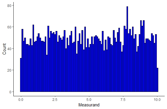
Figure \(\PageIndex{1}\): Random/Uniform Sample Distribution.
As expected we see in this distribution each measurand value has an equal probability of being observed/measured. This type of distribution is somewhat uncommon experimentally unless you are looking at a component of a Markov process typically in a simulation system but this type of distribution can be observed.
Exponential or Negative Exponential Distribution
The exponential distribution is typically valid for processes in which events occur continuously and independently at a constant average rate. Such a distribution is rare to find in real-world experimental scenarios however it does capture well some physical systems such as the time until a radioactive particle decays, or the time until default on payment to debt hold in some financial models.

Figure \(\PageIndex{2}\): Exponential Distribution.
The exponential distribution can be described as
\begin{equation}
f(x) = \lambda \exp^{-\lambda x}
\end{equation}
where the population mean is represented as \(\frac{1}{\lambda}\) as the standard deviation.
Poisson Distribution
The Poisson distribution is actually a discrete probability distribution, i.e. cannot be described by a continuous function. This distribution can be very useful to model the number and size of meteorites that hit the earth as well as modeling student exam score distributions. We can actually see the distrubution below
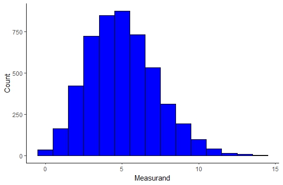
Figure \(\PageIndex{3}\): Poisson Distribution.
Binomial Distribution
The binomial distribution is another distribution that is discrete and this distribution fits random number generators extremely well. This distribution can be seen below
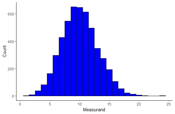
Figure \(\PageIndex{4}\): Binomial Distribution.
Log-Normal Distribution
The Log-normal distribution is a continuous distribution and also can be referred to as the Galton’s distribution. Unlike our previous distributions the Log-Normal distribution describes many natural phenomenon including the length of chess games, sizes of living tissues, many hydrology phenomenon, and many other phenomenon, which can be seen below

Figure \(\PageIndex{5}\): Log-Normal Distribution
The distribution can be described as seen below:
\begin{equation}
f(x) = \frac{1}{x \sigma \sqrt{2 \pi}}\exp \bigg ( - \frac{(\ln x - \mu)^2 }{2 \sigma^2} \bigg)
\end{equation}
Beta Distribution
The beta distribution is another continuous probability distribution and is defined by two parameters α and β which change the shape of the distribution as seen below
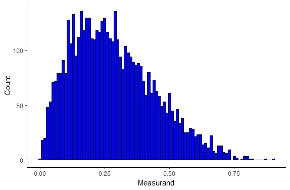
Figure \(\PageIndex{6}\): Beta Distribution
The distribution can be described as
\begin{equation}
f(x) = \frac{1}{B} x^{\alpha -1} (1-x)^{\beta -1}
\end{equation}
where B is a normalization factor. The beta distribution describes population genetics specifically allele frequencies, project management models, and other systems.
Gamma Distribution
The gamma distribution is another continuous distribution that can be described by two parameters and can be seen below
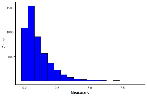
Figure \(\PageIndex{7}\): Gamma Distribution
The gamma distribution model describes the size of insurance claims and rainfall quite well as well as the age distribution of cancer incidences. The gamma distribution can be described as
\begin{equation}
f(x) = \frac{1}{B \beta^\alpha} x^{\alpha -1} \exp^{-\frac{x}{\beta}}
\end{equation}
where B is a constant normalization factor.
Weibull Distribution
The Weibull distribution is another continuous probability distribution governed by two parameters and this distribution famously describes fatigue failure of materials extremely well as well as many other physical systems and this distribution can be seen below
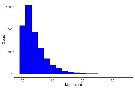
Figure \(\PageIndex{8}\): Weibull Distribution
Gaussian and Normal Distribution
One of the most common distribution that you will encounter is the Gaussian distribution, often referred to as the normal distribution or bell-curve, which can be seen below

Figure \(\PageIndex{9}\): Probability density function (PDF) or normal distribution curve. Notice the width of the Gaussian increases from blue to green.
The Gaussian will capture a myriad of physical systems and is by far the most likely distribution you will work with. Now remember, we are limited to working with samples of a population because it is either impractical or impossible to work with entire population however let us consider an infinite population of data, each datum representing a measurement of a single quantity, and assume that each datum, x, differs in magnitude only as a result of precision error. The probability of obtaining a specific value x depends on both the magnitude and distribution of x-values as described by the probability density function or PDF.
Since the population is infinite the PDF is a continuous curve. The PDF represents the probability of occurrence per unit change of x. The probability of measuring agiven x is not f(x) instead the probability of measuring an x in the interval \(\delta x = x_{2}-x_{1}\) is the area under the curve or:
\begin{equation}
P_{x_{1} \rightarrow x_{2}} = \int_{x_{1}}^{x_{2}} f(x) dx
\end{equation}
In any measurement some value of x must be observed so the total area under the curve is unity, 1, or alternatively the probability of measuring one value of x is 100% or equivalently
\begin{equation}
P = \int_{-\infty}^{\infty} f(x) dx = 1
\end{equation}
The form of the Gaussian Probability Density Function can be seen below
\begin{equation}
f(x) = \frac{1}{\sigma \sqrt{2 \pi}} \exp\bigg[- \frac{(x - \mu)^{2}}{2 \sigma^{2}}\bigg]
\end{equation}
where x is the magnitude of particular measurement, µ is the mean value of the entire population, and σ is the standard deviation of the entire population. µ is an unknown since the population is infinite.
Outliers
You have probably hear about outlier data points, i.e. data points that are much much higher or lower than the mean. There can be some controversy as an engineers in making the decision to neglect or disregard outlier data points. Typically in this class you can disregard a data point as illegitimate if the data point exceeds 3σ. However, it is good practice to always show this data point in your graphs and explain that when fitting a curve or determining a trend you disregarded this data point, do not just delete this point. The only time you can delete data you gather is if there was illegitimate error in which case all data must be disregarded and you must perform the experiment again.
We can simplify the form of the Gaussian PDF by defining an arbitrary variable z
\begin{equation}
z = \frac{x - \mu}{\sigma}
\end{equation}
and the resulting Gaussian PDF becomes
\begin{equation}
f(z) = \frac{1}{\sigma \sqrt{2 \pi}} e^{\frac{-z^{2}}{2}}
\end{equation}
The above definition is the standard curve and using tables or graphical integration you can determine the area under the standard curve between 0 and various values of z.
Once we have this equation we can then estimate the size of errors with various levels of confidence. For example let us consider the most common confidence interval that you may encounter, the 95% confidence interval. One way we can quantify error is to make the statement that with 95% confidence if I make a measurement (stress for example) that measurement will fall between these two bounds. What we are saying here is that 95% of the measurements of a population should fall between these two bounds. So to calculate these bounds we can simply solve for the bounds where we will find 90, 95, or 99% of our data or whatever confidence interval that we are working with as seen in the Mathematica notebook below

Figure \(\PageIndex{10}\): Solved Confidence interval bounds in terms of \(x \times \sigma\) for confidence intervals of 90,95, and 99%.
If you do not want to use mathematica you can instead use integration tables or for this function, Z-Tables as seen below. It should be noted that the table below lists values for only half the curve but since the standard curve is symmetric you can just multiply by 2 to get the total area. These tabulated values of areas is called the Z-distribution
Example Problems Confidence Intervals
Working with Z Tables
• What is the area under the standard normal distribution curve between z = −1.43 and 1.43?
• What percent of the population lies within this range?
• What range of z will contain 90% of the data?
Running and Tumbling E.coli
We measured the velocity of E.coli 135 times using Able Particle Tracker. The mean velocity was determined to be 3\(\mu m\) and the standard deviation was determined to be 0.1\(\mu m\). I’m particularly interested in velocity measurements between 2.857 and 3.143\(\frac{\mu m}{s}\), specifically the percentage of the population that will fall within this range because I plan to claim in my Nature paper that 95% of this data will fall within this range.
• What assumptions are you making about the data set?
– Assume normal distribution
• Calculate z for this data set?
• What is the area under the Standard Normal Distribution for this data set range?
• What percent of my data will fall within this range?
• How many measurements fall within this range?
• What range of velocities will contain 95% of the data?
Marble Diameters
I have a bag of marbles and I grab a sample of 765 marbles. From this sample I measure the diameters and find that the population mean is 200mm, the population standard deviation is 20mm. I need the range of marble diameters where I can expect to find 60% of the marbles in the population.
Ultimate Tensile Strength Measurements
I’m working at a Materials company and I have measured the UTS for a new material to have a µ = 303MPa and the σ = 33MPa. What is the probability I find a sample that exceeds a UTS of 350MPa.
Voltage Measurements
I’m measuring the voltage in my Helmholtz Coil apparatus and I find, after 150 exhausting measurements, that the population mean is 10V with a population standard deviation of 3.4. How many voltage measurements will fall between 10-15 volts?
Under Pressure Measurements
I’m measuring the pressure in a cylindrical pressure vessel and find that µ = 39Pa and σ = 4Pa. I took 120 measurements. How many measurements will fall between 35-45Pa? How many less than 35? How many less than 45?