
Chapter 4: Central Limit Theorem and Confidence Intervals for Large and Small Sample Sizes
- Page ID
- 99695
\( \newcommand{\vecs}[1]{\overset { \scriptstyle \rightharpoonup} {\mathbf{#1}} } \)
\( \newcommand{\vecd}[1]{\overset{-\!-\!\rightharpoonup}{\vphantom{a}\smash {#1}}} \)
\( \newcommand{\dsum}{\displaystyle\sum\limits} \)
\( \newcommand{\dint}{\displaystyle\int\limits} \)
\( \newcommand{\dlim}{\displaystyle\lim\limits} \)
\( \newcommand{\id}{\mathrm{id}}\) \( \newcommand{\Span}{\mathrm{span}}\)
( \newcommand{\kernel}{\mathrm{null}\,}\) \( \newcommand{\range}{\mathrm{range}\,}\)
\( \newcommand{\RealPart}{\mathrm{Re}}\) \( \newcommand{\ImaginaryPart}{\mathrm{Im}}\)
\( \newcommand{\Argument}{\mathrm{Arg}}\) \( \newcommand{\norm}[1]{\| #1 \|}\)
\( \newcommand{\inner}[2]{\langle #1, #2 \rangle}\)
\( \newcommand{\Span}{\mathrm{span}}\)
\( \newcommand{\id}{\mathrm{id}}\)
\( \newcommand{\Span}{\mathrm{span}}\)
\( \newcommand{\kernel}{\mathrm{null}\,}\)
\( \newcommand{\range}{\mathrm{range}\,}\)
\( \newcommand{\RealPart}{\mathrm{Re}}\)
\( \newcommand{\ImaginaryPart}{\mathrm{Im}}\)
\( \newcommand{\Argument}{\mathrm{Arg}}\)
\( \newcommand{\norm}[1]{\| #1 \|}\)
\( \newcommand{\inner}[2]{\langle #1, #2 \rangle}\)
\( \newcommand{\Span}{\mathrm{span}}\) \( \newcommand{\AA}{\unicode[.8,0]{x212B}}\)
\( \newcommand{\vectorA}[1]{\vec{#1}} % arrow\)
\( \newcommand{\vectorAt}[1]{\vec{\text{#1}}} % arrow\)
\( \newcommand{\vectorB}[1]{\overset { \scriptstyle \rightharpoonup} {\mathbf{#1}} } \)
\( \newcommand{\vectorC}[1]{\textbf{#1}} \)
\( \newcommand{\vectorD}[1]{\overrightarrow{#1}} \)
\( \newcommand{\vectorDt}[1]{\overrightarrow{\text{#1}}} \)
\( \newcommand{\vectE}[1]{\overset{-\!-\!\rightharpoonup}{\vphantom{a}\smash{\mathbf {#1}}}} \)
\( \newcommand{\vecs}[1]{\overset { \scriptstyle \rightharpoonup} {\mathbf{#1}} } \)
\(\newcommand{\longvect}{\overrightarrow}\)
\( \newcommand{\vecd}[1]{\overset{-\!-\!\rightharpoonup}{\vphantom{a}\smash {#1}}} \)
\(\newcommand{\avec}{\mathbf a}\) \(\newcommand{\bvec}{\mathbf b}\) \(\newcommand{\cvec}{\mathbf c}\) \(\newcommand{\dvec}{\mathbf d}\) \(\newcommand{\dtil}{\widetilde{\mathbf d}}\) \(\newcommand{\evec}{\mathbf e}\) \(\newcommand{\fvec}{\mathbf f}\) \(\newcommand{\nvec}{\mathbf n}\) \(\newcommand{\pvec}{\mathbf p}\) \(\newcommand{\qvec}{\mathbf q}\) \(\newcommand{\svec}{\mathbf s}\) \(\newcommand{\tvec}{\mathbf t}\) \(\newcommand{\uvec}{\mathbf u}\) \(\newcommand{\vvec}{\mathbf v}\) \(\newcommand{\wvec}{\mathbf w}\) \(\newcommand{\xvec}{\mathbf x}\) \(\newcommand{\yvec}{\mathbf y}\) \(\newcommand{\zvec}{\mathbf z}\) \(\newcommand{\rvec}{\mathbf r}\) \(\newcommand{\mvec}{\mathbf m}\) \(\newcommand{\zerovec}{\mathbf 0}\) \(\newcommand{\onevec}{\mathbf 1}\) \(\newcommand{\real}{\mathbb R}\) \(\newcommand{\twovec}[2]{\left[\begin{array}{r}#1 \\ #2 \end{array}\right]}\) \(\newcommand{\ctwovec}[2]{\left[\begin{array}{c}#1 \\ #2 \end{array}\right]}\) \(\newcommand{\threevec}[3]{\left[\begin{array}{r}#1 \\ #2 \\ #3 \end{array}\right]}\) \(\newcommand{\cthreevec}[3]{\left[\begin{array}{c}#1 \\ #2 \\ #3 \end{array}\right]}\) \(\newcommand{\fourvec}[4]{\left[\begin{array}{r}#1 \\ #2 \\ #3 \\ #4 \end{array}\right]}\) \(\newcommand{\cfourvec}[4]{\left[\begin{array}{c}#1 \\ #2 \\ #3 \\ #4 \end{array}\right]}\) \(\newcommand{\fivevec}[5]{\left[\begin{array}{r}#1 \\ #2 \\ #3 \\ #4 \\ #5 \\ \end{array}\right]}\) \(\newcommand{\cfivevec}[5]{\left[\begin{array}{c}#1 \\ #2 \\ #3 \\ #4 \\ #5 \\ \end{array}\right]}\) \(\newcommand{\mattwo}[4]{\left[\begin{array}{rr}#1 \amp #2 \\ #3 \amp #4 \\ \end{array}\right]}\) \(\newcommand{\laspan}[1]{\text{Span}\{#1\}}\) \(\newcommand{\bcal}{\cal B}\) \(\newcommand{\ccal}{\cal C}\) \(\newcommand{\scal}{\cal S}\) \(\newcommand{\wcal}{\cal W}\) \(\newcommand{\ecal}{\cal E}\) \(\newcommand{\coords}[2]{\left\{#1\right\}_{#2}}\) \(\newcommand{\gray}[1]{\color{gray}{#1}}\) \(\newcommand{\lgray}[1]{\color{lightgray}{#1}}\) \(\newcommand{\rank}{\operatorname{rank}}\) \(\newcommand{\row}{\text{Row}}\) \(\newcommand{\col}{\text{Col}}\) \(\renewcommand{\row}{\text{Row}}\) \(\newcommand{\nul}{\text{Nul}}\) \(\newcommand{\var}{\text{Var}}\) \(\newcommand{\corr}{\text{corr}}\) \(\newcommand{\len}[1]{\left|#1\right|}\) \(\newcommand{\bbar}{\overline{\bvec}}\) \(\newcommand{\bhat}{\widehat{\bvec}}\) \(\newcommand{\bperp}{\bvec^\perp}\) \(\newcommand{\xhat}{\widehat{\xvec}}\) \(\newcommand{\vhat}{\widehat{\vvec}}\) \(\newcommand{\uhat}{\widehat{\uvec}}\) \(\newcommand{\what}{\widehat{\wvec}}\) \(\newcommand{\Sighat}{\widehat{\Sigma}}\) \(\newcommand{\lt}{<}\) \(\newcommand{\gt}{>}\) \(\newcommand{\amp}{&}\) \(\definecolor{fillinmathshade}{gray}{0.9}\)So far we have been calculating confidence intervals assuming that we know the population mean and standard deviation. But this is often never possible to do. Instead, recall that we will take measurements or samples and attempt to get an estimate or an approximate measure of population mean and standard deviation from our sample measurements. And we also want to infer the probability distribution of the population from the sample. Let’s start our journey on how we can accomplish this.
Here you can find a series of pre-recorded lecture videos that cover this content: https://youtube.com/playlist?list=PL...A9jQYH4GX6Ojeg
Microwalker Rolling Velocity
As an undergraduate I performed experiments with super-paramagnetic particles and measured the velocity of the rolling particles my advisor was extremely and thorough to his undergraduate researchers so I had to measure the velocity of 138 particles. We predicted that the walkers would exhibit a mean velocity of 3\(\frac{\mu m}{s}\) and that the walker velocity should not deviate by more than 0.5\(\frac{\mu m}{s}\). The velocity measurements can be seen in the Mathematica Notebook below

Figure \(\PageIndex{1}\): Rolling Velocity of Microwalkers in \(\frac{\mu m}{s}\).
So can we prove at a 95% confidence interval that the walker velocity will not deviate more than 0.5\(\frac{\mu m}{s}\)?
Well we have a lot of data so let’s take a look at the data to make sure that our implicit assumption that we are working with a normally distributed population, i.e. Gaussian distribution. Let’s plot the data in a histogram. Does this distribution look Gaussian? You may be wondering if there is a quantitative method to determine whether a distribution is Gaussian or not and the short answer yes and we will get to this in a few lectures.
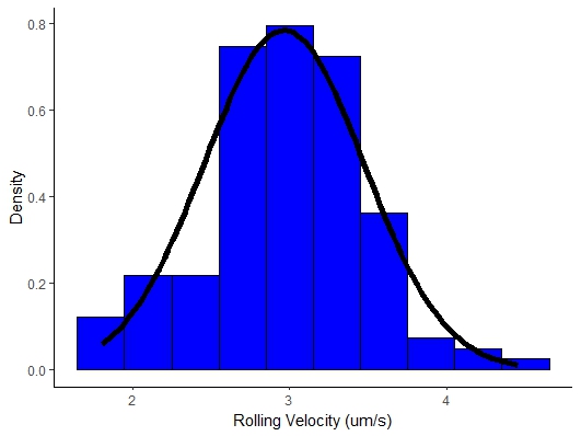
Figure \(\PageIndex{2}\): Microwalker Rolling Velocity Histogram.
Let’s calculate the sample mean and standard deviation and we find that
\begin{eqnarray}
\overline{x} = 3.041031\\
S_x = 0.5176254
\end{eqnarray}
So you can see as anticipated the sample mean and standard deviation are slightly different from the assumed population mean and standard deviation.
So to see if we do not deviate more than 0.5\(\frac{\mu m}{s}\) we can simply approximate the uncertainty in the population mean as follows:
\begin{equation}
\mu \pm 1.96 \sigma
\end{equation}
![]() Since we are working with a large sample size, n > 30 we can use the following approximation that x ≈ µ and that Sx ≈ σ so that we find that
Since we are working with a large sample size, n > 30 we can use the following approximation that x ≈ µ and that Sx ≈ σ so that we find that
\begin{equation}
\mu \pm 1.96 \sigma \approx \overline{x} \pm 1.96 S_x = 2.94 \pm 1.014546
\end{equation}
So we will in fact deviate more in this experiment.
Can we disregard 1.6 \(\frac{\mu m}{s}\) as an illegitimate data point or outlier? Justify.
Central Limit Theorem
We just examined the dispersion of sample values around the mean value of the sample, x. But we did not obtain an estimate for the uncertainty in x approximated to the true mean µ. To do this we would have to repeat the experiment test and compare the x of each sample test. Thus we would also obtain a set of samples for the mean.
One of the most important and profound theories in statistics deals with this set of sample means and their distribution and is referred to as the Central Limit Theorem. So far we have been working on the assumption that the population that we are working with is normally distributed. While many times that may be true it is not always the case. Let think for instance if we were working with a uniform sample distribution like the one below
.jpeg?revision=1)
Figure \(\PageIndex{3}\): Uniform Sample Distribution.
At this point one might think we must give up and we cannot perform any data analysis...noooo we can make it.
Instead the Central Limit Theorem postulates a very powerful idea that regardless of the shape of the population distribution the distribution of the mean values of a sample will be normally distributed as long as you obtain a large value of means, n > 30. We can see this visually with an example in the Mathematica Notebook for this lecture. If we randomly pick 6 samples from this distribution and average if we look at 2 or 10 averages as seen below the distribution do not look Gaussian but if we select 30 or more (sometimes 20 is enough but I would obtain 30 just to be safe) then we see the distribution of the mean measurand values becomes Gaussian!!!
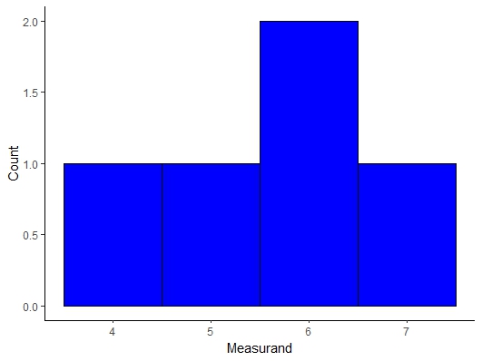
Figure \(\PageIndex{4}\): Uniform Distribution Mean Sample Distribution with 5 Mean Samples.
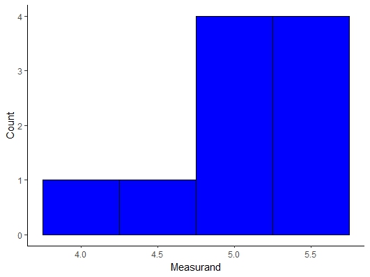
Figure \(\PageIndex{5}\): Uniform Distribution Mean Sample Distribution with 10 Mean Samples.
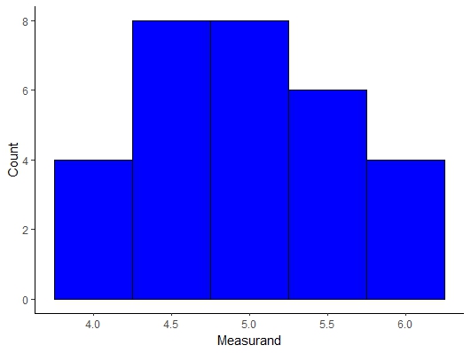
Figure \(\PageIndex{6}\): Uniform Distribution Mean Sample Distribution with 30 Mean Samples.
This has implications for the analysis we can perform but let’s prove this and show that it works for other types of distributions like an Exponential, χ2, and β. As you can see below the distribution of the means are clearly normal or Gaussian Distributions.
The practical application that is of interest to us as experimentalists is that we do not need to think about or worry about the shape of the population distribution. Since we know that the sample means are normally distributed we can simply use the normal distribution of the means to calculate confidence intervals and do more complex analysis and comparisons moving forward...you are so lucky t-test comparisons and hypothesis testing are coming soon!!!
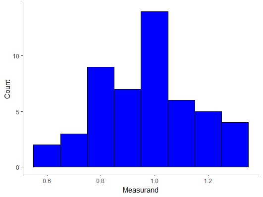
Figure \(\PageIndex{7}\): Mean Distribution of 50 Samples for Exponential Distributions.
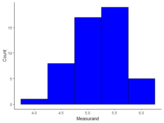
Figure \(\PageIndex{8}\): Mean Distribution of 50 Samples for Poisson Distributions.
So when we invoke the central limit theorem we can make the following definitions where the standard deviation of the distribution of the means is
\begin{equation}
S_{\overline{x}} = \frac{S_x}{\sqrt{n}}
\end{equation}
We can use the standard deviation of the means to now re-write our PDF or Gaussian function so z now becomes when describing the distribution of the means
\begin{equation}
z = \frac{\overline{x} - \mu}{S_{\overline{x}}} = \frac{\overline{x} - \mu}{\frac{S_x}{\sqrt{n}}}
\end{equation}
This new definition of z allows us to re-write our confidence interval equation as follows but now we can explicitly determine the confidence level or uncertainty that in the population mean!!!
\begin{equation}
\mu = \overline{x} \pm z_{\frac{c}{2}} \frac{S_x}{\sqrt{n}}
\end{equation}
Whew!! That was a lot of work now let’s go back to our rolling particles and calculate the 95% confidence interval for the population mean pressure.
Well that will simply be
\begin{equation}
\mu = \overline{x} \pm z_{\frac{c}{2}} \frac{S_x}{\sqrt{n}} = 3.041031 \pm 0.08636387
\end{equation}
As you can see this is a much much much smaller range than our previous calculation due to the \(\sqrt{\frac{1}{n}}\) factor. This is the key difference when trying to estimate the uncertainty in the population mean or using \(\overline{x}\)as an estimate of the population mean. Previously we were just looking at the likelihood of observing a value that deviates from the population mean by a particular value.
In summary the c% interval for the mean value is narrower than the data by a factor of \(\frac{1}{\sqrt{n}}\). This is because n observations have been used to average out the random deviations of individual measurements.
Confidence Intervals for Small Samples
We have been working with large samples thus far which is generally considered to be when n ≥ 30 but there are many experiments when n will often be less than 30. For these situations we will utilize the Student’s t-distribution, developed by an amateur statistician writing under the pseudonym Student:
\begin{equation}
t=\frac{\overline{x} - \mu}{\frac{S_{x}}{\sqrt{n}}}
\end{equation}
Student was actually William Gosset a Guinness brewer who was applying statistical analysis to the brewing process. Guinness was against him publishing the data and thus giving away the Guinness secrets so he published under the pseudonym.
The assumption here is that the underlying population satisfies the Gaussian distribution. This distribution also depends on the degrees of freedom, ν = n − 1.
t-distribution is similar to PDF, it is symmetric and the total area is unity. Moreover, the t-distribution approaches the standard Gaussian PDF as ν or n becomes large and for n > 30 the two distributions are identical as will be seen in the t-table soon.
The area beneath the t-distribution is tabulated at the end of these notes
The area, α, is between t and t →∞ and for a given sample sizes. This is very different from our Z-table where we were looking at the area between z=0 and z. α corresponds to the probability that for a given sample size, t will have a value greater than that given in the table. We can assert with c% = (1−α) that the actual value of t does not fall in the shaded area.
A two sided confidence interval is then:
\begin{equation}
\overline{x} - t_{\frac{\alpha}{2},\nu} \frac{S_{x}}{\sqrt{n}} < \mu < \overline{x} + t_{\frac{\alpha}{2},\nu} \frac{S_{x}}{\sqrt{n}}
\end{equation}
Sometimes α in literature will be referred to as the level of significance.
Designing Phase Change Materials
You are weighing out polymer samples to be integrated into a phase change material application to regulate temperature in textile applications. You are given 18 samples from your lab partner which should nominally be 2mg. You weight them and obtain the following results.
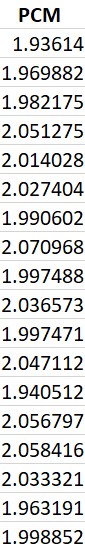
Figure \(\PageIndex{9}\): PCM Measurements.
Based on these sample and the assumption that the parent population is normally distributed, what is the 95% confidence interval for the population mean.
\begin{equation}
\mu = 2.009567 \pm 0.020387 mg
\end{equation}
Calculating Confidence Intervals in R
You can actually calculate confidence intervals in R directly using the t.test functionality and we can get the confidence interval as seen below
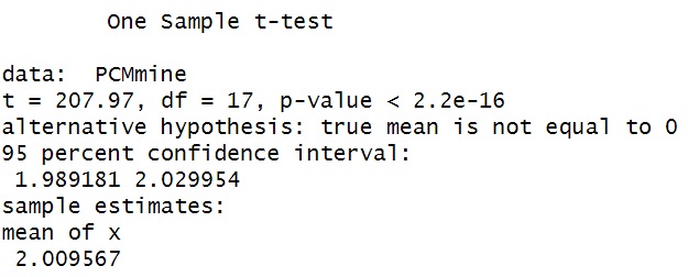
Figure \(\PageIndex{10}\): T-Test PCM Measurement.
and you can see that our results match our theoretical calculations which is fantastic!!!
But what is it do we see here about hypothesis tests??
Well we will discuss this next lecture, same bat time same bat place!