
Chapter 8: F-Tests and Variable Independence
- Page ID
- 99732
\( \newcommand{\vecs}[1]{\overset { \scriptstyle \rightharpoonup} {\mathbf{#1}} } \)
\( \newcommand{\vecd}[1]{\overset{-\!-\!\rightharpoonup}{\vphantom{a}\smash {#1}}} \)
\( \newcommand{\id}{\mathrm{id}}\) \( \newcommand{\Span}{\mathrm{span}}\)
( \newcommand{\kernel}{\mathrm{null}\,}\) \( \newcommand{\range}{\mathrm{range}\,}\)
\( \newcommand{\RealPart}{\mathrm{Re}}\) \( \newcommand{\ImaginaryPart}{\mathrm{Im}}\)
\( \newcommand{\Argument}{\mathrm{Arg}}\) \( \newcommand{\norm}[1]{\| #1 \|}\)
\( \newcommand{\inner}[2]{\langle #1, #2 \rangle}\)
\( \newcommand{\Span}{\mathrm{span}}\)
\( \newcommand{\id}{\mathrm{id}}\)
\( \newcommand{\Span}{\mathrm{span}}\)
\( \newcommand{\kernel}{\mathrm{null}\,}\)
\( \newcommand{\range}{\mathrm{range}\,}\)
\( \newcommand{\RealPart}{\mathrm{Re}}\)
\( \newcommand{\ImaginaryPart}{\mathrm{Im}}\)
\( \newcommand{\Argument}{\mathrm{Arg}}\)
\( \newcommand{\norm}[1]{\| #1 \|}\)
\( \newcommand{\inner}[2]{\langle #1, #2 \rangle}\)
\( \newcommand{\Span}{\mathrm{span}}\) \( \newcommand{\AA}{\unicode[.8,0]{x212B}}\)
\( \newcommand{\vectorA}[1]{\vec{#1}} % arrow\)
\( \newcommand{\vectorAt}[1]{\vec{\text{#1}}} % arrow\)
\( \newcommand{\vectorB}[1]{\overset { \scriptstyle \rightharpoonup} {\mathbf{#1}} } \)
\( \newcommand{\vectorC}[1]{\textbf{#1}} \)
\( \newcommand{\vectorD}[1]{\overrightarrow{#1}} \)
\( \newcommand{\vectorDt}[1]{\overrightarrow{\text{#1}}} \)
\( \newcommand{\vectE}[1]{\overset{-\!-\!\rightharpoonup}{\vphantom{a}\smash{\mathbf {#1}}}} \)
\( \newcommand{\vecs}[1]{\overset { \scriptstyle \rightharpoonup} {\mathbf{#1}} } \)
\( \newcommand{\vecd}[1]{\overset{-\!-\!\rightharpoonup}{\vphantom{a}\smash {#1}}} \)
\(\newcommand{\avec}{\mathbf a}\) \(\newcommand{\bvec}{\mathbf b}\) \(\newcommand{\cvec}{\mathbf c}\) \(\newcommand{\dvec}{\mathbf d}\) \(\newcommand{\dtil}{\widetilde{\mathbf d}}\) \(\newcommand{\evec}{\mathbf e}\) \(\newcommand{\fvec}{\mathbf f}\) \(\newcommand{\nvec}{\mathbf n}\) \(\newcommand{\pvec}{\mathbf p}\) \(\newcommand{\qvec}{\mathbf q}\) \(\newcommand{\svec}{\mathbf s}\) \(\newcommand{\tvec}{\mathbf t}\) \(\newcommand{\uvec}{\mathbf u}\) \(\newcommand{\vvec}{\mathbf v}\) \(\newcommand{\wvec}{\mathbf w}\) \(\newcommand{\xvec}{\mathbf x}\) \(\newcommand{\yvec}{\mathbf y}\) \(\newcommand{\zvec}{\mathbf z}\) \(\newcommand{\rvec}{\mathbf r}\) \(\newcommand{\mvec}{\mathbf m}\) \(\newcommand{\zerovec}{\mathbf 0}\) \(\newcommand{\onevec}{\mathbf 1}\) \(\newcommand{\real}{\mathbb R}\) \(\newcommand{\twovec}[2]{\left[\begin{array}{r}#1 \\ #2 \end{array}\right]}\) \(\newcommand{\ctwovec}[2]{\left[\begin{array}{c}#1 \\ #2 \end{array}\right]}\) \(\newcommand{\threevec}[3]{\left[\begin{array}{r}#1 \\ #2 \\ #3 \end{array}\right]}\) \(\newcommand{\cthreevec}[3]{\left[\begin{array}{c}#1 \\ #2 \\ #3 \end{array}\right]}\) \(\newcommand{\fourvec}[4]{\left[\begin{array}{r}#1 \\ #2 \\ #3 \\ #4 \end{array}\right]}\) \(\newcommand{\cfourvec}[4]{\left[\begin{array}{c}#1 \\ #2 \\ #3 \\ #4 \end{array}\right]}\) \(\newcommand{\fivevec}[5]{\left[\begin{array}{r}#1 \\ #2 \\ #3 \\ #4 \\ #5 \\ \end{array}\right]}\) \(\newcommand{\cfivevec}[5]{\left[\begin{array}{c}#1 \\ #2 \\ #3 \\ #4 \\ #5 \\ \end{array}\right]}\) \(\newcommand{\mattwo}[4]{\left[\begin{array}{rr}#1 \amp #2 \\ #3 \amp #4 \\ \end{array}\right]}\) \(\newcommand{\laspan}[1]{\text{Span}\{#1\}}\) \(\newcommand{\bcal}{\cal B}\) \(\newcommand{\ccal}{\cal C}\) \(\newcommand{\scal}{\cal S}\) \(\newcommand{\wcal}{\cal W}\) \(\newcommand{\ecal}{\cal E}\) \(\newcommand{\coords}[2]{\left\{#1\right\}_{#2}}\) \(\newcommand{\gray}[1]{\color{gray}{#1}}\) \(\newcommand{\lgray}[1]{\color{lightgray}{#1}}\) \(\newcommand{\rank}{\operatorname{rank}}\) \(\newcommand{\row}{\text{Row}}\) \(\newcommand{\col}{\text{Col}}\) \(\renewcommand{\row}{\text{Row}}\) \(\newcommand{\nul}{\text{Nul}}\) \(\newcommand{\var}{\text{Var}}\) \(\newcommand{\corr}{\text{corr}}\) \(\newcommand{\len}[1]{\left|#1\right|}\) \(\newcommand{\bbar}{\overline{\bvec}}\) \(\newcommand{\bhat}{\widehat{\bvec}}\) \(\newcommand{\bperp}{\bvec^\perp}\) \(\newcommand{\xhat}{\widehat{\xvec}}\) \(\newcommand{\vhat}{\widehat{\vvec}}\) \(\newcommand{\uhat}{\widehat{\uvec}}\) \(\newcommand{\what}{\widehat{\wvec}}\) \(\newcommand{\Sighat}{\widehat{\Sigma}}\) \(\newcommand{\lt}{<}\) \(\newcommand{\gt}{>}\) \(\newcommand{\amp}{&}\) \(\definecolor{fillinmathshade}{gray}{0.9}\)Here you can find a series of pre-recorded lecture videos that cover this content: https://youtube.com/playlist?list=PLSKNWIzCsmjDNUfe0P58VkcTtwIfxpSw2&si=Xrau1wfJKX8-ZI-k
Analyzing Samples Based on Variance
We have previously discussed the \(\chi^2\) goodness of fit test but we want to build upon our ANOVA analysis which looked at analyzing populations based on variances and build upon that and introduce a new statistical tool, specifically the \(\chi^2\) test. Here our key test metric for this type of test
\begin{equation}
\chi^2 = \frac{(n-1)S^2}{\sigma_o^2}
\end{equation}
where σo is our null population standard deviation and S is our sample standard deviation previously defined. We can use this test just as we have for other statistical measures and for hypothesis testing as well, in fact let’s go ahead and work with our old material A and test to see if this sample comes from a population with a standard deviation of 1.31 GPa at a 95% confidence interval.
\begin{eqnarray}
H_{0}: \sigma = 1.31 GPa \\
H_{a}: \sigma \neq 1.31 GPa \\
\chi^2 = \frac{(n-1)S^2}{\sigma_o^2} =8.58\\
\chi_{0.05,11}^{2} = 19.675
\end{eqnarray}
Here we can clearly see that we are in the do not reject regime. We can also see from our p-value is 0.68 which confirms we are in the reject regime.
We can also compare whether material B comes from a population with a standard deviation greater than 1.7 GPa at a 99% confidence interval?
\begin{eqnarray}
H_{0}: \sigma = 1.7 GPa \\
H_{a}: \sigma > 1.7 GPa \\
\chi^2 = \frac{(n-1)S^2}{\sigma_o^2} =22.05\\
\chi_{0.01,14}^{2} = 29.141
\end{eqnarray}
Here we can clearly see that we are in the do not reject regime. We can also see from our p-value is 0.078 which confirms we are in the reject regime.
However, as we have demonstrated several times in this course we often want to make statements to compare samples and to do this we have to invoke the F-Test to compare variances/standard deviations.
F-Test
One can also perform hypothesis testing on multiple samples by examining variances and this can be done using the F-Test metric as defined below
\begin{equation}
F = \frac{S_1^2}{S_2^2}
\end{equation}
We can run a hypothesis test with this as well, let’s go ahead and keep examining our material A and B at a 95% confidence interval.
\begin{eqnarray}
H_{0}: \sigma_A^2 = \sigma_B^2 \\
H_{a}: \sigma_A^2 \neq \sigma_B^2 \\
F = \frac{S_A^2}{S_B^2} = 0.29 \\
\end{eqnarray}
We can look up the theoretical F value but we can see from the p-value of 0.04798 and we are in the do not reject region because this is a two-sided test so the critical p-value is 0.025.
We can also run a test to see if the variance of A is smaller than B at a 90% confidence level
\begin{eqnarray}
H_{0}: \sigma_A^2 = \sigma_B^2 \\
H_{a}: \sigma_A^2 < \sigma_B^2 \\
F = \frac{S_A^2}{S_B^2} = 0.29 \\
\end{eqnarray}
We are in the reject region as the p-value is 0.02!
\(\chi^2\) Test of Independence
We can look for correlations between variables and specifically we can see whether variables are independent or dependent. The test works just the same as the goodness of fit test in that we will be comparing the observed frequencies to the expected frequencies.
Typically when performing these types of test the data can will be reported in a table not too dissimilar to the one we can see here below
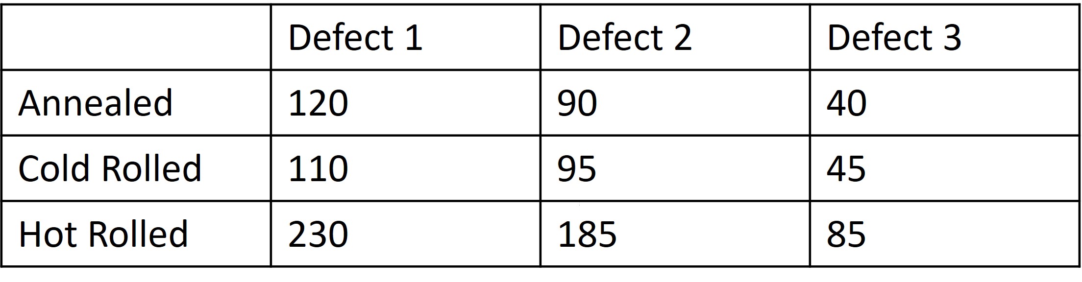.jpg?revision=1)
Figure \(\PageIndex{1}\): Material Processing Steps and Defects.
Here we are looking at 500 samples and classifying if the sample exhibits a particular type of defect, 1-3. We also correlate that sample according to the type of material processing step that was undergone for that particular sample. Now one question
that we may ask ourselves is if there is a correlation between the material process and the defect that occurs in the sample.
We can then calculate the expected frequencies by multiplying the total number of observations for the row and the total number of observations for the column divided by the total number of observations.
Thus we will be looking effectively at a probability and one can find the relationship that
\begin{equation}
\sum_{i_1}^r p_{ij} = 1
\end{equation}
where r is the number of rows and pij is the probability of obtaining an observation belonging to the ith row and jth column.
Luckily, our \(\chi^2\) expression is similar with one caveat
\begin{equation}
\chi^{2} = \sum \limits_{i=1}^r \sum_{j}^c \frac{(O_{ij} - E_{ij})^2}{E_{ij}}
\end{equation}
where here \(r\) is the number of rows and \(c\) is the number of columns in our table. Additionally, our degrees of freedom \(\nu = (r-1)(c-1)\).
Therefore we can perform our hypothesis testing procedures at a 95% confidence interval
\begin{eqnarray}
H_{0}: p_{ij} = \sum_{i=1}^c \sum_{j=1}^c p_{ij} \\
H_{a}: p_{ij} \neq \sum_{i=1}^c \sum_{j=1}^c p_{ij} \\
\chi^{2} = \sum \limits_{i=1}^r \sum_{j}^c \frac{(O_{ij} - E_{ij})^2}{E_{ij}} = 0.86404 \\
\chi^{2}_{0.05,4} = 9.488
\end{eqnarray}
So we can see that we are in the Do Not Reject regime and our p-value confirms this as well!!
We can also confirm this by hand calculations as well.