
5.3: Mesh Analysis
- Page ID
- 52919

\( \newcommand{\vecs}[1]{\overset { \scriptstyle \rightharpoonup} {\mathbf{#1}} } \)
\( \newcommand{\vecd}[1]{\overset{-\!-\!\rightharpoonup}{\vphantom{a}\smash {#1}}} \)
\( \newcommand{\dsum}{\displaystyle\sum\limits} \)
\( \newcommand{\dint}{\displaystyle\int\limits} \)
\( \newcommand{\dlim}{\displaystyle\lim\limits} \)
\( \newcommand{\id}{\mathrm{id}}\) \( \newcommand{\Span}{\mathrm{span}}\)
( \newcommand{\kernel}{\mathrm{null}\,}\) \( \newcommand{\range}{\mathrm{range}\,}\)
\( \newcommand{\RealPart}{\mathrm{Re}}\) \( \newcommand{\ImaginaryPart}{\mathrm{Im}}\)
\( \newcommand{\Argument}{\mathrm{Arg}}\) \( \newcommand{\norm}[1]{\| #1 \|}\)
\( \newcommand{\inner}[2]{\langle #1, #2 \rangle}\)
\( \newcommand{\Span}{\mathrm{span}}\)
\( \newcommand{\id}{\mathrm{id}}\)
\( \newcommand{\Span}{\mathrm{span}}\)
\( \newcommand{\kernel}{\mathrm{null}\,}\)
\( \newcommand{\range}{\mathrm{range}\,}\)
\( \newcommand{\RealPart}{\mathrm{Re}}\)
\( \newcommand{\ImaginaryPart}{\mathrm{Im}}\)
\( \newcommand{\Argument}{\mathrm{Arg}}\)
\( \newcommand{\norm}[1]{\| #1 \|}\)
\( \newcommand{\inner}[2]{\langle #1, #2 \rangle}\)
\( \newcommand{\Span}{\mathrm{span}}\) \( \newcommand{\AA}{\unicode[.8,0]{x212B}}\)
\( \newcommand{\vectorA}[1]{\vec{#1}} % arrow\)
\( \newcommand{\vectorAt}[1]{\vec{\text{#1}}} % arrow\)
\( \newcommand{\vectorB}[1]{\overset { \scriptstyle \rightharpoonup} {\mathbf{#1}} } \)
\( \newcommand{\vectorC}[1]{\textbf{#1}} \)
\( \newcommand{\vectorD}[1]{\overrightarrow{#1}} \)
\( \newcommand{\vectorDt}[1]{\overrightarrow{\text{#1}}} \)
\( \newcommand{\vectE}[1]{\overset{-\!-\!\rightharpoonup}{\vphantom{a}\smash{\mathbf {#1}}}} \)
\( \newcommand{\vecs}[1]{\overset { \scriptstyle \rightharpoonup} {\mathbf{#1}} } \)
\(\newcommand{\longvect}{\overrightarrow}\)
\( \newcommand{\vecd}[1]{\overset{-\!-\!\rightharpoonup}{\vphantom{a}\smash {#1}}} \)
\(\newcommand{\avec}{\mathbf a}\) \(\newcommand{\bvec}{\mathbf b}\) \(\newcommand{\cvec}{\mathbf c}\) \(\newcommand{\dvec}{\mathbf d}\) \(\newcommand{\dtil}{\widetilde{\mathbf d}}\) \(\newcommand{\evec}{\mathbf e}\) \(\newcommand{\fvec}{\mathbf f}\) \(\newcommand{\nvec}{\mathbf n}\) \(\newcommand{\pvec}{\mathbf p}\) \(\newcommand{\qvec}{\mathbf q}\) \(\newcommand{\svec}{\mathbf s}\) \(\newcommand{\tvec}{\mathbf t}\) \(\newcommand{\uvec}{\mathbf u}\) \(\newcommand{\vvec}{\mathbf v}\) \(\newcommand{\wvec}{\mathbf w}\) \(\newcommand{\xvec}{\mathbf x}\) \(\newcommand{\yvec}{\mathbf y}\) \(\newcommand{\zvec}{\mathbf z}\) \(\newcommand{\rvec}{\mathbf r}\) \(\newcommand{\mvec}{\mathbf m}\) \(\newcommand{\zerovec}{\mathbf 0}\) \(\newcommand{\onevec}{\mathbf 1}\) \(\newcommand{\real}{\mathbb R}\) \(\newcommand{\twovec}[2]{\left[\begin{array}{r}#1 \\ #2 \end{array}\right]}\) \(\newcommand{\ctwovec}[2]{\left[\begin{array}{c}#1 \\ #2 \end{array}\right]}\) \(\newcommand{\threevec}[3]{\left[\begin{array}{r}#1 \\ #2 \\ #3 \end{array}\right]}\) \(\newcommand{\cthreevec}[3]{\left[\begin{array}{c}#1 \\ #2 \\ #3 \end{array}\right]}\) \(\newcommand{\fourvec}[4]{\left[\begin{array}{r}#1 \\ #2 \\ #3 \\ #4 \end{array}\right]}\) \(\newcommand{\cfourvec}[4]{\left[\begin{array}{c}#1 \\ #2 \\ #3 \\ #4 \end{array}\right]}\) \(\newcommand{\fivevec}[5]{\left[\begin{array}{r}#1 \\ #2 \\ #3 \\ #4 \\ #5 \\ \end{array}\right]}\) \(\newcommand{\cfivevec}[5]{\left[\begin{array}{c}#1 \\ #2 \\ #3 \\ #4 \\ #5 \\ \end{array}\right]}\) \(\newcommand{\mattwo}[4]{\left[\begin{array}{rr}#1 \amp #2 \\ #3 \amp #4 \\ \end{array}\right]}\) \(\newcommand{\laspan}[1]{\text{Span}\{#1\}}\) \(\newcommand{\bcal}{\cal B}\) \(\newcommand{\ccal}{\cal C}\) \(\newcommand{\scal}{\cal S}\) \(\newcommand{\wcal}{\cal W}\) \(\newcommand{\ecal}{\cal E}\) \(\newcommand{\coords}[2]{\left\{#1\right\}_{#2}}\) \(\newcommand{\gray}[1]{\color{gray}{#1}}\) \(\newcommand{\lgray}[1]{\color{lightgray}{#1}}\) \(\newcommand{\rank}{\operatorname{rank}}\) \(\newcommand{\row}{\text{Row}}\) \(\newcommand{\col}{\text{Col}}\) \(\renewcommand{\row}{\text{Row}}\) \(\newcommand{\nul}{\text{Nul}}\) \(\newcommand{\var}{\text{Var}}\) \(\newcommand{\corr}{\text{corr}}\) \(\newcommand{\len}[1]{\left|#1\right|}\) \(\newcommand{\bbar}{\overline{\bvec}}\) \(\newcommand{\bhat}{\widehat{\bvec}}\) \(\newcommand{\bperp}{\bvec^\perp}\) \(\newcommand{\xhat}{\widehat{\xvec}}\) \(\newcommand{\vhat}{\widehat{\vvec}}\) \(\newcommand{\uhat}{\widehat{\uvec}}\) \(\newcommand{\what}{\widehat{\wvec}}\) \(\newcommand{\Sighat}{\widehat{\Sigma}}\) \(\newcommand{\lt}{<}\) \(\newcommand{\gt}{>}\) \(\newcommand{\amp}{&}\) \(\definecolor{fillinmathshade}{gray}{0.9}\)In some respects mesh analysis is a mirror of nodal analysis. While nodal analysis leverages KCL to create a series of node equations that are used to solve for node voltages, mesh analysis uses KVL to create a series of loop equations that can be solved for mesh currents. A mesh current should not be confused with a branch current. While branch currents represent the current flowing through a particular component, mesh currents combine to create branch currents. That is, the current through any particular component may be an individual mesh current or a combination of two mesh currents. Circuits using complex series-parallel arrangement with multiple voltage and/or current sources may be solved using this technique. It is, however, limited to planar circuits. Planar circuits are those that can be drawn on a flat plane without having any of their wires cross. In essence, these circuits can be drawn so that they appear like a series of window panes. Non-planar circuits may be 3D in appearance and in such a circuit it becomes impossible to define the loop equations as any given component might have more than two meshing currents.
General Method
Consider the circuit of Figure 7.3.1 . We begin by designating a series of loops. These loops should be minimal in size and cover all components at least once. By convention, the loops are drawn clockwise. There is nothing magic about them being clockwise, it is just a matter of consistency. The current path along a loop is referred to as a mesh current. In the circuit of Figure 7.3.1 we have two loops, and thus, two mesh currents, \(I_1\) and \(I_2\). Note that all components exist in at least one loop (and sometimes in more than one loop, like \(R_3\)). Depending on circuit values, one or more of these loop's directions may in fact be opposite of reality. This is not a problem. If this is the case, the currents will show up as negative values, and thus we know that they're really flowing counter-clockwise.
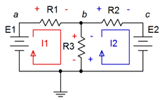
Figure 7.3.1 : Circuit for mesh analysis.
We begin by writing KVL equations for each loop.
\[\text{Loop 1: } E_1 = \text{ voltage across } R_1 + \text{ voltage across } R_3 \nonumber \]
\[\text{Loop 2: }−E_2 = \text{ voltage across } R_2 + \text{ voltage across } R_3 \nonumber \]
\[(E_2 \text{ is negative as } I_2 \text{ is drawn flowing out of its negative terminal.)} \nonumber \]
Expand the voltage terms using Ohm's law.
\[\text{Loop 1: } E_1 = I_1 \cdot R_1 + (I_1 − I_2) R_3 \nonumber \]
\[\text{Loop 2: } −E_2 = I_2 \cdot R_2 + (I_2 − I_1) R_3 \nonumber \]
Expanding and collecting terms yields:
\[\text{Loop 1: } E_1 = (R_1 + R_3) I_1 − R_3 \cdot I_2 \nonumber \]
\[\text{Loop 2: }: −E_2 = R_3 \cdot I_1 + (R_2 + R_3) I_2 \nonumber \]
Assuming that the resistor values and source voltages are known, we have two equations with two unknowns. These can be solved for \(I_1\) and \(I_2\) using simultaneous equation solution techniques such as determinants or Gauss-Jordan elimination.
Find \(V_b\) and \(V_{bc}\) for the circuit of Figure 7.3.2 .
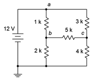
Figure 7.3.2 : Circuit for Example 7.3.1 .
The first step is to define a set of clockwise loops that are of minimum size and which cover all components. These loops are drawn in Figure 7.3.3 . Also, the polarities of the voltage drops produced by these currents are drawn next to the components in the same color for easy identification. Note that some components see only one current, such as the 3 k\( \Omega \) resistor that sees only \(I_2\); and some see two currents in opposing directions, such the 5 k\( \Omega \) resistor that sees both \(I_2\) and \(I_3\). With multiple current directions flowing through a single component, obeying the resulting voltage polarities becomes very important.
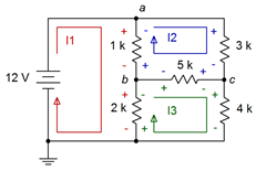
Figure 7.3.3 : Circuit of Example 7.3.1 with current loops and polarities added.
We now write KVL summations around each loop. If the current passing through a component sees a polarity of + to − then this is counted as a voltage drop while the reverse counts as a voltage rise. This is true even for voltage sources (i.e., a voltage source may appear negative in one loop and positive in another).
\[\sum V_{rises} = \sum V_{drops} \nonumber \]
\[\text{Loop 1: } 12 V = V_{1k}+V_{2k} \nonumber \]
\[\text{Loop 2: } 0V = V_{3k}+V_{5k}+V_{1k} \nonumber \]
\[\text{Loop 3: } 0V = V_{5k}+V_{4k}+V_{2k} \nonumber \]
These are expanded using Ohm's law. The current for the loop under consideration is deemed positive while any opposing (i.e., meshing) current is deemed negative:
\[\text{Loop 1: } 12 V = 1k(I_1 −I_2 )+2 k(I_1 −I_2 ) \nonumber \]
\[\text{Loop 2: } 0V = 3 k(I_2 )+5k(I_2 −I_3 )+1k(I_2 −I_1 ) \nonumber \]
\[\text{Loop 3: } 0V = 5 k(I_3 −I_2 )+4k(I_3 )+2k(I_3 −I_1 ) \nonumber \]
The terms are expanded:
\[\text{Loop 1: } 12 V = 1k I_1 −1 k I_2+2 k I_1 −2 k I_3 \nonumber \]
\[\text{Loop 2: } 0V = 3 k I_2+5k I_2 −5k I_3+1k I_2 −1 k I_1 \nonumber \]
\[\text{Loop 3: } 0V = 5 k I_3 −5k I_2+4k I_3+2k I_3 −2k I_1 \nonumber \]
Like terms are grouped, once again creating aligned columns for the current coefficients:
\[\text{Loop 1: } 12 V = (1k+2k)I_1 −1 k I_2 −2 k I_3 \nonumber \]
\[\text{Loop 2: } 0V = −1k I_1+(3 k+5k+1k) I_2 −5k I_3 \nonumber \]
\[\text{Loop 3: } 0V = −2k I_1 −5k I_2+(5k+4k+2k)I_3 \nonumber \]
Which simplifies to:
\[\text{Loop 1: } 12 V = 3k I_1 −1k I_2 −2 k I_3 \nonumber \]
\[\text{Loop 2: } 0V = −1k I_1 +9 k I_2 −5k I_3 \nonumber \]
\[\text{Loop 3: } 0V = −2k I_1 −5k I_2+11 k I_3 \nonumber \]
Note that we have diagonal symmetry. The solution is \(I_1\) = 5.729 mA, \(I_2\) = 1.6258 mA and \(I_3\) = 1.7806 mA. To find \(V_b\) we need to find the net current through the 2 k\( \Omega \) resistor. That's \(I_1 − I_3\), or 5.729 mA − 1.7806 mA, which is 3.9484 mA. When multiplied by 2 k\( \Omega \) we find \(V_b\) = 7.8968 volts. Similarly, \(V_{bc} = (I_3 − I_2)\) 5 k\( \Omega \) = (1.7806 mA − 1.6258 mA ) 5 k\( \Omega \), or 774 mV.
Computer Simulation
In order to verify the results of the analysis, the circuit is entered into a simulator and a virtual voltmeter is placed across the 5 k\( \Omega \) resistor. This is shown in Figure 7.3.4 . The results agree nicely with the original analysis.
As nice as this is, in a practical circuit we need to be concerned about the effects of component tolerance. It would be extraordinarily odd if during production each resistor was equal to precisely the nominal value specified. In reality, each resistor will have a stated tolerance. Thus, with all five resistors changing slightly from unit to unit, we should expect the currents and voltages to vary as well. The question is, what would be a typical spread? This can be addressed via a Monte Carlo analysis. This analysis is, in fact, a series of simulations. Each simulation uses randomized component values that fall within the stated tolerance spread. For example, if we specify that the 1 k\( \Omega \) resistor has a 5% tolerance, then the actual resistor used for a simulation will be a randomly generated value between 950 \( \Omega \) and 1050 \( \Omega \). We then state how many trials we'd like, each one using their own unique randomized values for each component.
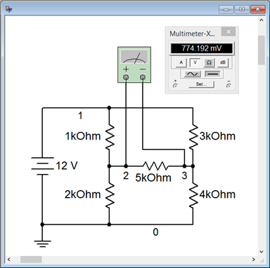
Figure 7.3.4 : Circuit of Figure 7.3.2 in a simulator with a virtual voltmeter.
The results of a Monte Carlo analysis using the DC operating point simulation is shown in Figure 7.3.5 . Ten randomized trials were generated for the value of \(V_b\). Each of the five resistors was assigned a tolerance of 5%. As can be seen, voltage values both above and below the nominal simulation can result.
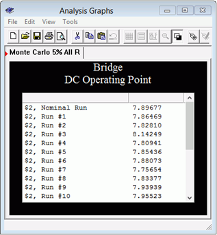
Figure 7.3.5 : Monte Carlo analysis results for the circuit of Figure 7.3.2 .
Inspection Method
Like nodal analysis, there is a method to generate the equations by inspection. Simply focus on one loop, which we'll call the loop under inspection, and ask the following questions: what is the total source voltage in this loop? This yields the voltage constant for the equation. Then sum all of the resistance values in the loop under inspection. This yields the coefficient for that current term. For the remaining current coefficients in this equation, sum the resistances that are in common between the loop under inspection and the other loops, respectively. These values will always be negative. Repeat this process for all loops, with each loop in turn becoming the loop under inspection. As was the case with nodal analysis, the set of equations produced must exhibit diagonal symmetry, that is, if a diagonal is drawn from the upper left to the lower right through the \(I_R\) pairs, then the coefficients found above the diagonal will have to match those found below the diagonal.
While it is possible to extend this technique to include current sources, it is often easier and less error-prone to convert the current sources into voltage sources and continue with the direct inspection method outlined above. Either way, it is important to remember that the number of loops determines the number of equations to be solved.
Find \(V_c\) for the circuit of Figure 7.3.6 .
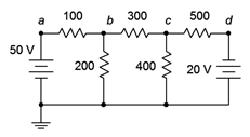
Figure 7.3.6 : Circuit for Example 7.3.2 .
First, we'll label the loops, as shown in Figure 7.3.7 .
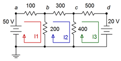
Figure 7.3.7 : Circuit of Example 7.3.2 with current loops identified.
Now, beginning with loop 1, sum all of the voltage sources in this loop. That's +50 volts. Secondly, sum all of the resistors in this loop. That's 100 \( \Omega \) + 200 \( \Omega \), or 300 \( \Omega \). This is the coefficient for the \(I_1\) term. The coefficient for the \(I_2\) term is the sum of all resistances that are in common between loops 1 and 2. That's just the 200 \( \Omega \) resistor. The coefficient for the \(I_3\) term would be the sum of all resistances that are in common between loop 1 and loop 3. In this circuit, there aren't any so the coefficient is zero. The first equation is:
\[\text{Loop 1: } 50 V = 300I_1 −200I_2 −0I_3 \nonumber \]
Repeat the process for loops 2 and 3:
\[\text{Loop 2: } 0V = −200I_1 +900I_2 −400I_3 \nonumber \]
\[\text{Loop 3: } 20V = −0I_1 −400I_2 +900I_3 \nonumber \]
Note that the 20 volt source shows up positive because of the direction of \(I_3\) (into the negative terminal and out of the positive terminal).
As required, we have diagonal symmetry. The solution is \(I_1\) = 214.47 mA, \(I_2\) = 71.698 mA and \(I_3\) = 54.088 mA. \(V_c\) is the net current through the 400 \( \Omega \) resistor times 400 \( \Omega \). The net current is \(I_2 − I_3\), or 71.698 mA − 54.088 mA, which is 17.61 mA. When multiplied by 400 \( \Omega \) we find \(V_b\) = 7.044 volts. Note that we use \(I_2 − I_3\) and not \(I_3 − I_2\). The reason is because we are trying to find the voltage from node \(c\) to ground, and \(I_2\) is the current flowing in that direction. In contrast, using \(I_3 − I_2\) would yield the voltage from ground to node \(c\); the same magnitude but opposite sign.
As a crosscheck, KVL states that \(V_c + V_{500}\) has to equal the −20 volt source. The drop across the 500 \( \Omega \) is 54.088 mA times 500 \( \Omega \), or 27.044 volts from left to right. Starting at node \(c\) of 7.044 volts and then dropping 27.044 volts yields − 20 volts as expected.
Supermesh
Sometimes you may run across a current source which has no associated internal resistance, such as found in the circuit of Figure 7.3.8 . This is similar to the situation seen previously under nodal analysis where a voltage source does not have a specified internal resistance. There are two ways of solving this predicament. The first is add a very large resistance in parallel with the current source and then perform a source conversion on the pair so that the inspection method of mesh can be followed. The larger the value of this resistor, the more accuracy that is obtained. As a general rule it should be, at minimum, at least a couple of orders of magnitude larger than any surrounding resistor, and preferably larger. The second method is to use supermesh. A supermesh is a larger mesh loop than contains other mesh loops inside of it.
Consider the circuit shown in Figure 7.3.8 . In the center we have a current source, \(I_s\), which lacks an associated internal resistance. Two traditional mesh loops, \(I_1\) and \(I_2\), are labeled as usual. The problem here is that we cannot use an Ohm's law based \(IR\) voltage drop for \(V_b\). We have no way to express this as the voltage across \(I_s\) is an unknown. On the other hand, what we do know is that \(I_s\) must equal the combination of the traditional mesh currents \(I_1\) and \(I_2\). That is, from the perspective of the first loop, \(I_s = I_1 − I_2\). Remember, one or both of the mesh currents could be negative, and thus rotating counterclockwise.
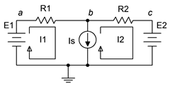
Figure 7.3.8 : Circuit for supermesh.
At this point we invoke the idea of a supermesh loop. First, we replace the offending current source with its ideal internal resistance (an open). The supermesh loop is drawn which encompasses the original two loops. This is shown in Figure 7.3.9 . The supermesh loop is drawn in red and labeled.
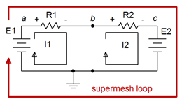
Figure 7.3.9 : Supermesh labeled.
We now perform a KVL summation around the supermesh loop, similar to what we have done previously. The difference this time is that we need to recognize that components each see one of the original mesh currents; namely \(I_1\) or \(I_2\) in this case. We do not solve for a supermesh current, we simply use the supermesh to define the loop for the KVL summation. The summation follows:
\[ \sum V_{rises} = \sum V_{drops} \nonumber \]
\[E_1 = V_{R1}+V_{R2}+E_2 \nonumber \]
The voltage drops across the resistors can be expanded using Ohm's law, using the original mesh current associated with each resistor.
\[E_1 −E_2 = I_1 R_1+I_2 R_2 \nonumber \]
By inspection,
\[I_s = I_1 −I_2 \text{ or} \nonumber \]
\[I_2 = I_1 −I_s \nonumber \]
We now have two equations with two unknowns and can solve for \(I_1\) and \(I_2\). This procedure is illustrated in the following example.
Find \(V_b\) for the circuit of Figure 7.3.10 .
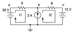
Figure 7.3.10 : Circuit for Example 7.3.3 .
First, we'll label the loops, as shown in Figure 7.3.11 .
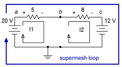
Figure 7.3.11 : Circuit of Figure 7.3.10 with supermesh labeled.
Next, we'll perform a KVL summation around the supermesh loop.
\[\sum V_{rises} = \sum V_{drops} \nonumber \]
\[20 V = V_{R1}+V_{R2} +12V \nonumber \]
Expand using Ohm's law and rearrange:
\[20 V −12 V = 5 \Omega I_1+8 \Omega I_2 \nonumber \]
\[8V = 5 \Omega I_1+8 \Omega I_2 \nonumber \]
By inspection we know
\[3A = I_2 −I_1 \text{ or} \nonumber \]
\[I_2 = I_1+3A \nonumber \]
We can substitute this expression into the prior supermesh expression and solve for I1:
\[8 V = 5 \Omega I_1+8 \Omega I_2 \nonumber \]
\[8 V = 5 \Omega I_1+8 \Omega (I_1+3A) \nonumber \]
\[8 V = 5 \Omega I_1+8 \Omega I_1+24 V \nonumber \]
\[−16 V = 13 \Omega I_1 \nonumber \]
\[I_1 \approx−1.231A \nonumber \]
Thus, \(I_2\) = −1.231 A + 3 A, or 1.769 A. To determine \(V_b\) we simply subtract the drop across the 5 \( \Omega \) resistor from the 20 volt source.
\[V_b = 20 V − I_1 5 \Omega \nonumber \]
\[V_b = 20 V − (−1.231 A)5 \Omega \nonumber \]
\[V_b \approx 26.15 V \nonumber \]
As a crosscheck, we could also add the voltage across the 8 \( \Omega \) resistor to the 12 volt source:
\[V_b = 12V +I_2 8 \Omega \nonumber \]
\[V_b = 12V +1.769 A 8 \Omega \nonumber \]
\[V_b \approx26.15 V \nonumber \]
Comparison of Nodal and Mesh
Compared to nodal analysis, mesh analysis has the advantage of dealing with resistances rather than conductances when writing the system of equations. Further, the mesh inspection method works with voltage sources which tends to be convenient for many circuits, while the nodal inspection method requires current sources. On the down side, the resulting set of mesh currents requires further processing in order to find either branch currents or node voltages, while nodal analysis produces node voltages directly with no further processing. Mesh also has the disadvantage of being limited to planar circuits while there are no such limits to nodal.