
8.2: Activity 2 - Binary Search Tree
- Page ID
- 47927

\( \newcommand{\vecs}[1]{\overset { \scriptstyle \rightharpoonup} {\mathbf{#1}} } \)
\( \newcommand{\vecd}[1]{\overset{-\!-\!\rightharpoonup}{\vphantom{a}\smash {#1}}} \)
\( \newcommand{\id}{\mathrm{id}}\) \( \newcommand{\Span}{\mathrm{span}}\)
( \newcommand{\kernel}{\mathrm{null}\,}\) \( \newcommand{\range}{\mathrm{range}\,}\)
\( \newcommand{\RealPart}{\mathrm{Re}}\) \( \newcommand{\ImaginaryPart}{\mathrm{Im}}\)
\( \newcommand{\Argument}{\mathrm{Arg}}\) \( \newcommand{\norm}[1]{\| #1 \|}\)
\( \newcommand{\inner}[2]{\langle #1, #2 \rangle}\)
\( \newcommand{\Span}{\mathrm{span}}\)
\( \newcommand{\id}{\mathrm{id}}\)
\( \newcommand{\Span}{\mathrm{span}}\)
\( \newcommand{\kernel}{\mathrm{null}\,}\)
\( \newcommand{\range}{\mathrm{range}\,}\)
\( \newcommand{\RealPart}{\mathrm{Re}}\)
\( \newcommand{\ImaginaryPart}{\mathrm{Im}}\)
\( \newcommand{\Argument}{\mathrm{Arg}}\)
\( \newcommand{\norm}[1]{\| #1 \|}\)
\( \newcommand{\inner}[2]{\langle #1, #2 \rangle}\)
\( \newcommand{\Span}{\mathrm{span}}\) \( \newcommand{\AA}{\unicode[.8,0]{x212B}}\)
\( \newcommand{\vectorA}[1]{\vec{#1}} % arrow\)
\( \newcommand{\vectorAt}[1]{\vec{\text{#1}}} % arrow\)
\( \newcommand{\vectorB}[1]{\overset { \scriptstyle \rightharpoonup} {\mathbf{#1}} } \)
\( \newcommand{\vectorC}[1]{\textbf{#1}} \)
\( \newcommand{\vectorD}[1]{\overrightarrow{#1}} \)
\( \newcommand{\vectorDt}[1]{\overrightarrow{\text{#1}}} \)
\( \newcommand{\vectE}[1]{\overset{-\!-\!\rightharpoonup}{\vphantom{a}\smash{\mathbf {#1}}}} \)
\( \newcommand{\vecs}[1]{\overset { \scriptstyle \rightharpoonup} {\mathbf{#1}} } \)
\( \newcommand{\vecd}[1]{\overset{-\!-\!\rightharpoonup}{\vphantom{a}\smash {#1}}} \)
\(\newcommand{\avec}{\mathbf a}\) \(\newcommand{\bvec}{\mathbf b}\) \(\newcommand{\cvec}{\mathbf c}\) \(\newcommand{\dvec}{\mathbf d}\) \(\newcommand{\dtil}{\widetilde{\mathbf d}}\) \(\newcommand{\evec}{\mathbf e}\) \(\newcommand{\fvec}{\mathbf f}\) \(\newcommand{\nvec}{\mathbf n}\) \(\newcommand{\pvec}{\mathbf p}\) \(\newcommand{\qvec}{\mathbf q}\) \(\newcommand{\svec}{\mathbf s}\) \(\newcommand{\tvec}{\mathbf t}\) \(\newcommand{\uvec}{\mathbf u}\) \(\newcommand{\vvec}{\mathbf v}\) \(\newcommand{\wvec}{\mathbf w}\) \(\newcommand{\xvec}{\mathbf x}\) \(\newcommand{\yvec}{\mathbf y}\) \(\newcommand{\zvec}{\mathbf z}\) \(\newcommand{\rvec}{\mathbf r}\) \(\newcommand{\mvec}{\mathbf m}\) \(\newcommand{\zerovec}{\mathbf 0}\) \(\newcommand{\onevec}{\mathbf 1}\) \(\newcommand{\real}{\mathbb R}\) \(\newcommand{\twovec}[2]{\left[\begin{array}{r}#1 \\ #2 \end{array}\right]}\) \(\newcommand{\ctwovec}[2]{\left[\begin{array}{c}#1 \\ #2 \end{array}\right]}\) \(\newcommand{\threevec}[3]{\left[\begin{array}{r}#1 \\ #2 \\ #3 \end{array}\right]}\) \(\newcommand{\cthreevec}[3]{\left[\begin{array}{c}#1 \\ #2 \\ #3 \end{array}\right]}\) \(\newcommand{\fourvec}[4]{\left[\begin{array}{r}#1 \\ #2 \\ #3 \\ #4 \end{array}\right]}\) \(\newcommand{\cfourvec}[4]{\left[\begin{array}{c}#1 \\ #2 \\ #3 \\ #4 \end{array}\right]}\) \(\newcommand{\fivevec}[5]{\left[\begin{array}{r}#1 \\ #2 \\ #3 \\ #4 \\ #5 \\ \end{array}\right]}\) \(\newcommand{\cfivevec}[5]{\left[\begin{array}{c}#1 \\ #2 \\ #3 \\ #4 \\ #5 \\ \end{array}\right]}\) \(\newcommand{\mattwo}[4]{\left[\begin{array}{rr}#1 \amp #2 \\ #3 \amp #4 \\ \end{array}\right]}\) \(\newcommand{\laspan}[1]{\text{Span}\{#1\}}\) \(\newcommand{\bcal}{\cal B}\) \(\newcommand{\ccal}{\cal C}\) \(\newcommand{\scal}{\cal S}\) \(\newcommand{\wcal}{\cal W}\) \(\newcommand{\ecal}{\cal E}\) \(\newcommand{\coords}[2]{\left\{#1\right\}_{#2}}\) \(\newcommand{\gray}[1]{\color{gray}{#1}}\) \(\newcommand{\lgray}[1]{\color{lightgray}{#1}}\) \(\newcommand{\rank}{\operatorname{rank}}\) \(\newcommand{\row}{\text{Row}}\) \(\newcommand{\col}{\text{Col}}\) \(\renewcommand{\row}{\text{Row}}\) \(\newcommand{\nul}{\text{Nul}}\) \(\newcommand{\var}{\text{Var}}\) \(\newcommand{\corr}{\text{corr}}\) \(\newcommand{\len}[1]{\left|#1\right|}\) \(\newcommand{\bbar}{\overline{\bvec}}\) \(\newcommand{\bhat}{\widehat{\bvec}}\) \(\newcommand{\bperp}{\bvec^\perp}\) \(\newcommand{\xhat}{\widehat{\xvec}}\) \(\newcommand{\vhat}{\widehat{\vvec}}\) \(\newcommand{\uhat}{\widehat{\uvec}}\) \(\newcommand{\what}{\widehat{\wvec}}\) \(\newcommand{\Sighat}{\widehat{\Sigma}}\) \(\newcommand{\lt}{<}\) \(\newcommand{\gt}{>}\) \(\newcommand{\amp}{&}\) \(\definecolor{fillinmathshade}{gray}{0.9}\)Introduction
A binary tree is made of nodes, where each node contains a left pointer, a right pointer, and a data element also called a key. The root pointer points to the topmost node in the tree. The left and right pointers recursively points to left and right sub-tree respectively. A null pointer represents a binary tree with no elements, that is, an empty tree. Figure 2.2.1 depicts a binary tree.
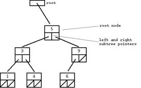
A binary search tree (BST) also called an ordered binary tree is a type of binary tree where the nodes are arranged in order. That is, for each node, all elements in its left sub-tree are less-or-equal to its element, and all the elements in its right sub-tree are greater than its element. The tree shown in Figure 2.2.1 is a binary search tree since the root node element is a 5, and its left sub-tree elements (i.e., 1, 3, 4) are less than 5, and its right sub-tree elements (i.e., 6, 9) are greater than 5. Recursively, each of the sub-trees must also obey the binary search tree constraint, that is, in the (1, 3, 4) sub-tree, the node with element 3 is the root, and that 1 <= 3 and 4 > 3. In this regard, note that a binary search tree is different from a binary tree. The nodes at the bottom edge of the tree which have empty sub-trees and are called leaf nodes (i.e., 1, 4, 6), while the others are called internal nodes (i.e., 3, 5, 9).
Activity Details
A binary tree is recursively defined as follows:
- An empty tree is a binary tree
- A node with two child sub-trees is a binary tree
- Only what you get from (i) by a finite number of applications of (ii) is a binary tree.
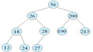
Now check whether Figure 2.2.2 is a binary tree.

A binary search tree (BST) is a fundamental data structure that can support dynamic set operations including: Search, Minimum, Maximum, Predecessor, Successor, Insert, and Delete. The efficiency of its operations (especially, the search and insert operations) make it be suited to use of building dictionaries and priority queues. Its basic operations take time proportional to the height, h, of the tree: i.e., O(h).
Like a binary tree, binary search tree is represented by a linked data structure of nodes. The root (T) points to the root of tree T. Each node contains three fields: key, left (pointer to left child/root of left sub-tree) and right (pointer to right child/root of right sub-tree).
A binary tree is a binary search tree if the stored keys satisfy the following two binary search tree properties:
- ∀ y in left sub-tree of x, then key[y] ≤ key[x].
- ∀ y in right sub-tree of x, then key[y] ≥ key[x].
Do the keys of the binary tree in Figure 2.2.3 satisfy binary search tree properties?
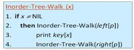
A binary search tree property allows its keys to be recursively visited/printed in monotonically increasing order, called an in-order traversal (walk). Figure 2.2.4 presents a pseudo-code for the in-order traversal. The correctness of the in-order walk can be elaborated through induction approach on the size of tree as follows: For an empty tree (i.e., size=0), this is easy. Suppose size >1, then
- Prints left sub-tree in order by induction
- Prints root, which comes after all elements in left sub-tree (still in order)
- Prints right sub-tree in order (all elements come after root, so still in order)
Recall that all dynamic set search operations on a binary search tree can be supported in O(h) time, where h is the tree height. Note that h = Θ(lg n) for a balanced binary tree (and for an average tree built by adding nodes in random order) and that h = Θ(n) for an unbalanced tree that resembles a linear chain of n nodes in the worst case.
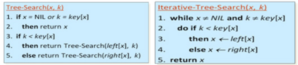
In the following we present the algorithms for some of the dynamic set operations. In Figure 2.2.5 and 2.2.6 presents the algorithms for the tree search operation. Figure 2.2.5 presents the algorithm for the search operation using both the recursive and iterative method respectively. The running time for both algorithms is O(h). However, the iterative tree search method is more efficient on most computers, while the recursive tree search is elegantly straightforward.
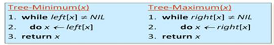
The other important dynamic set operation is finding Minimum and Maximum key respectively. The binary search tree properties guarantees that the minimum key is located at the left-most node and the maximum key is located at the right-most node. Figure 2.2.6 presents the algorithm for finding minimum and maximum keys.
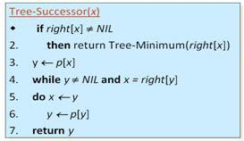
The other dynamic set operations on a binary search tree are finding the Predecessor and Successor keys. The successor of node x is the node y such that key[y] is the smallest key greater than key[x]. The successor of the largest key is NIL. The search for successor key consists of two cases:
- If node x has a non-empty right sub-tree, then x’s successor is the minimum in the right sub-tree of x.
- If node x has an empty right sub-tree, then
- As long as we move to the left up the tree (move up through right children), we are visiting smaller keys.
- x’s successor y is the node that x is the predecessor of (x is the maximum in y’s left sub-tree).
That is, x’s successor y, is the lowest ancestor of x whose left child is also an ancestor of x.
Figure 2.2.7 presents the pseudo-code for the successor operation. The code for predecessor operation is symmetric. The running time is both cases is O(h).
Insertion is also an important dynamic set operation on binary search tree. The insertion operation changes the dynamic set represented by a BST. The operation should ensure the binary search tree properties holds after a change. Generally, insertion is easier than deletion. Figure 2.2.8 presents the pseudo-code for insertion operation.

The analysis of insertion operation is as follows:
- Initialization takes O(1)
- The while loop in lines 3-7 searches for place to insert z, maintaining parent y. This takes O(h) time.
- Lines 8-13 insert the value in O(1).
Thus, overall it takes O(h) time to insert a node.
The delete operation in a BST is somehow involving. The BST deletion operation Tree-Delete (T, x) considers three cases:
- case 0 : if x has no children then remove x
- case 1 : if x has one child then make p[x] point to child
- case 2 : if x has two children (sub-trees), then swap x with its successor and perform case 0 or case 1 to delete it.
Overall delete operation takes O(h) time to delete a node. The pseudo-code for deleting a key in a BST is presented below:
Tree-Delete(T, z)
/* Determine which node to splice out: either z or z’s successor. */
if left[z] = NIL or right[z] = NIL
then y ← z
else y ← Tree-Successor[z]
/* Set x to a non-NIL child of x, or to NIL if y has no children. */
if left[y] ≠ NIL
then x ← left[y]
else x ← right[y]
/* y is removed from the tree by manipulating pointers of p[y] and x */
if x ≠ NIL
then p[x] ← p[y]
if p[y] = NIL
then root[T] ← x
else if y ← left[p[i]]
then left[p[y]] ← x
else right[p[y]] ← x
/* If z’s successor was spliced out, copy its data into z */
if y ≠ z
then key[z] ← key[y]
copy y’s satellite data into z.
return y
How do we know that case 2 should go to case 0 or case 1 instead of back to case 2? Due to the fact that when x has 2 children, its successor is the minimum in its right sub-tree, and that successor has no left child (hence 0 or 1 child). Equivalently, we could swap with predecessor instead of successor. It might be good to alternate to avoid creating unbalanced tree.
Conclusion
In this activity binary search trees were presented. Binary search trees is among advanced data structures of practical interest due to the efficiency of its basic operations including search and insert that make it attractive for implementing dictionaries and priority queues.
- Explain each of the following terms:
- Binary tree
- Binary search tree
- In-order tree traversal
- Draw the BST that results when you insert items with keys
A F R I C A N V I R T U A L U N I V E R S I T Y
in that order into an initially empty tree.
- Suppose we have integer values between 1 and 1000 in a BST and search for 363. Which of the following cannot be the sequence of keys examined (Hint: Draw the BST as if you were tracing the keys in the order given).
- 2 252 401 398 330 363
- 399 387 219 266 382 381 278 363
- 3 923 220 911 244 898 258 362 363
- 4 924 278 347 621 299 392 358 363
- 5 925 202 910 245 363