
9.3: Activity 3 - Sorting Algorithms by Merge and Partition methods
- Page ID
- 47933

\( \newcommand{\vecs}[1]{\overset { \scriptstyle \rightharpoonup} {\mathbf{#1}} } \)
\( \newcommand{\vecd}[1]{\overset{-\!-\!\rightharpoonup}{\vphantom{a}\smash {#1}}} \)
\( \newcommand{\id}{\mathrm{id}}\) \( \newcommand{\Span}{\mathrm{span}}\)
( \newcommand{\kernel}{\mathrm{null}\,}\) \( \newcommand{\range}{\mathrm{range}\,}\)
\( \newcommand{\RealPart}{\mathrm{Re}}\) \( \newcommand{\ImaginaryPart}{\mathrm{Im}}\)
\( \newcommand{\Argument}{\mathrm{Arg}}\) \( \newcommand{\norm}[1]{\| #1 \|}\)
\( \newcommand{\inner}[2]{\langle #1, #2 \rangle}\)
\( \newcommand{\Span}{\mathrm{span}}\)
\( \newcommand{\id}{\mathrm{id}}\)
\( \newcommand{\Span}{\mathrm{span}}\)
\( \newcommand{\kernel}{\mathrm{null}\,}\)
\( \newcommand{\range}{\mathrm{range}\,}\)
\( \newcommand{\RealPart}{\mathrm{Re}}\)
\( \newcommand{\ImaginaryPart}{\mathrm{Im}}\)
\( \newcommand{\Argument}{\mathrm{Arg}}\)
\( \newcommand{\norm}[1]{\| #1 \|}\)
\( \newcommand{\inner}[2]{\langle #1, #2 \rangle}\)
\( \newcommand{\Span}{\mathrm{span}}\) \( \newcommand{\AA}{\unicode[.8,0]{x212B}}\)
\( \newcommand{\vectorA}[1]{\vec{#1}} % arrow\)
\( \newcommand{\vectorAt}[1]{\vec{\text{#1}}} % arrow\)
\( \newcommand{\vectorB}[1]{\overset { \scriptstyle \rightharpoonup} {\mathbf{#1}} } \)
\( \newcommand{\vectorC}[1]{\textbf{#1}} \)
\( \newcommand{\vectorD}[1]{\overrightarrow{#1}} \)
\( \newcommand{\vectorDt}[1]{\overrightarrow{\text{#1}}} \)
\( \newcommand{\vectE}[1]{\overset{-\!-\!\rightharpoonup}{\vphantom{a}\smash{\mathbf {#1}}}} \)
\( \newcommand{\vecs}[1]{\overset { \scriptstyle \rightharpoonup} {\mathbf{#1}} } \)
\( \newcommand{\vecd}[1]{\overset{-\!-\!\rightharpoonup}{\vphantom{a}\smash {#1}}} \)
\(\newcommand{\avec}{\mathbf a}\) \(\newcommand{\bvec}{\mathbf b}\) \(\newcommand{\cvec}{\mathbf c}\) \(\newcommand{\dvec}{\mathbf d}\) \(\newcommand{\dtil}{\widetilde{\mathbf d}}\) \(\newcommand{\evec}{\mathbf e}\) \(\newcommand{\fvec}{\mathbf f}\) \(\newcommand{\nvec}{\mathbf n}\) \(\newcommand{\pvec}{\mathbf p}\) \(\newcommand{\qvec}{\mathbf q}\) \(\newcommand{\svec}{\mathbf s}\) \(\newcommand{\tvec}{\mathbf t}\) \(\newcommand{\uvec}{\mathbf u}\) \(\newcommand{\vvec}{\mathbf v}\) \(\newcommand{\wvec}{\mathbf w}\) \(\newcommand{\xvec}{\mathbf x}\) \(\newcommand{\yvec}{\mathbf y}\) \(\newcommand{\zvec}{\mathbf z}\) \(\newcommand{\rvec}{\mathbf r}\) \(\newcommand{\mvec}{\mathbf m}\) \(\newcommand{\zerovec}{\mathbf 0}\) \(\newcommand{\onevec}{\mathbf 1}\) \(\newcommand{\real}{\mathbb R}\) \(\newcommand{\twovec}[2]{\left[\begin{array}{r}#1 \\ #2 \end{array}\right]}\) \(\newcommand{\ctwovec}[2]{\left[\begin{array}{c}#1 \\ #2 \end{array}\right]}\) \(\newcommand{\threevec}[3]{\left[\begin{array}{r}#1 \\ #2 \\ #3 \end{array}\right]}\) \(\newcommand{\cthreevec}[3]{\left[\begin{array}{c}#1 \\ #2 \\ #3 \end{array}\right]}\) \(\newcommand{\fourvec}[4]{\left[\begin{array}{r}#1 \\ #2 \\ #3 \\ #4 \end{array}\right]}\) \(\newcommand{\cfourvec}[4]{\left[\begin{array}{c}#1 \\ #2 \\ #3 \\ #4 \end{array}\right]}\) \(\newcommand{\fivevec}[5]{\left[\begin{array}{r}#1 \\ #2 \\ #3 \\ #4 \\ #5 \\ \end{array}\right]}\) \(\newcommand{\cfivevec}[5]{\left[\begin{array}{c}#1 \\ #2 \\ #3 \\ #4 \\ #5 \\ \end{array}\right]}\) \(\newcommand{\mattwo}[4]{\left[\begin{array}{rr}#1 \amp #2 \\ #3 \amp #4 \\ \end{array}\right]}\) \(\newcommand{\laspan}[1]{\text{Span}\{#1\}}\) \(\newcommand{\bcal}{\cal B}\) \(\newcommand{\ccal}{\cal C}\) \(\newcommand{\scal}{\cal S}\) \(\newcommand{\wcal}{\cal W}\) \(\newcommand{\ecal}{\cal E}\) \(\newcommand{\coords}[2]{\left\{#1\right\}_{#2}}\) \(\newcommand{\gray}[1]{\color{gray}{#1}}\) \(\newcommand{\lgray}[1]{\color{lightgray}{#1}}\) \(\newcommand{\rank}{\operatorname{rank}}\) \(\newcommand{\row}{\text{Row}}\) \(\newcommand{\col}{\text{Col}}\) \(\renewcommand{\row}{\text{Row}}\) \(\newcommand{\nul}{\text{Nul}}\) \(\newcommand{\var}{\text{Var}}\) \(\newcommand{\corr}{\text{corr}}\) \(\newcommand{\len}[1]{\left|#1\right|}\) \(\newcommand{\bbar}{\overline{\bvec}}\) \(\newcommand{\bhat}{\widehat{\bvec}}\) \(\newcommand{\bperp}{\bvec^\perp}\) \(\newcommand{\xhat}{\widehat{\xvec}}\) \(\newcommand{\vhat}{\widehat{\vvec}}\) \(\newcommand{\uhat}{\widehat{\uvec}}\) \(\newcommand{\what}{\widehat{\wvec}}\) \(\newcommand{\Sighat}{\widehat{\Sigma}}\) \(\newcommand{\lt}{<}\) \(\newcommand{\gt}{>}\) \(\newcommand{\amp}{&}\) \(\definecolor{fillinmathshade}{gray}{0.9}\)Introduction
This activity will present two sorting algorithms. The first algorithm called merge sort is based on merge method, and the second algorithm called quick sort is based on partition method.
Activity Details
Merge Sort Algorithm
The Merge sort algorithm is based on the divide-and-conquer strategy. Its worst-case running time has a lower order of growth than insertion sort. Since the algorithm deals with sub-problems, we state each sub-problem as sorting a sub-array A[p .. r]. Initially, p = 1 and r = n, but these values change as recursion proceeds through sub-problems.
To sort A[p .. r], the merge sort algorithm proceeds as follows:
- Divide step - If a given array A has zero or one element, simply return as it is already sorted. Otherwise, split A[p .. r] into two sub-arrays A[p .. q] and A[q + 1 .. r], each containing about half of the elements of A[p .. r].
That is, q is the halfway point of A[p .. r].
- Conquer step - Conquer by recursively sorting the two sub-arrays A[p .. q] and A[q + 1 .. r].
- Combine step - Combine the elements back in A[p .. r] by merging the two sorted sub-arrays A[p .. q] and A[q + 1 .. r] into a sorted sequence. This step will be accomplished by procedure MERGE (A, p, q, r).
Note that the recursion ends when the sub-array has just one element, so that it is trivially sorted (base case). The following are the description of the merge sort algorithm: To sort the entire sequence A[1 .. n], make the initial call to the procedure MERGE-SORT (A, 1, n).
MERGE-SORT (A, p, r)
- IF p < r // Check for base case
- THEN q = FLOOR[(p + r)/2] // Divide step
- MERGE (A, p, q) // Conquer step
- MERGE (A, q + 1, r) // Conquer step
- MERGE (A, p, q, r) // Conquer step
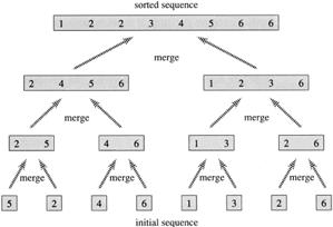
Figure 3.3.1 depicts a bottom-up view of the merge sort procedure for n = 8.
What remains is the MERGE procedure. The following is the input and output of the MERGE procedure.
INPUT - Array A and indices p, q, r such that p ≤ q ≤ r and sub-array A[p .. q] is sorted and sub-array A[q + 1 .. r] is sorted. By restrictions on p, q, r, neither sub-array is empty.
OUTPUT- The two sub-arrays are merged into a single sorted sub-array in A[p .. r].
The merge procedure takes Θ(n) time, where n = r − p + 1, which is the number of elements being merged. The idea behind linear time merging can be easily understood by thinking of two piles of cards; each pile is sorted and placed face-up on a table with the smallest cards on top. Merge these into a single sorted pile, face-down on the table, by completing the following basic steps:
- Choose the smaller of the two top cards.
- Remove it from its pile, thereby exposing a new top card.
- Place the chosen card face-down onto the output pile.
- Repeat steps 1 - 3 until one input pile is empty.
- Eventually, take the remaining input pile and place it face-down onto the output pile.
Each basic step takes constant time, i.e., O(1), since it involves checking the two top cards. There are at most n basic steps, since each basic step removes one card from the input piles, and we started with n cards in the input piles. Therefore, this procedure should take Θ(n) time.
Now the question is do we actually need to check whether a pile is empty before each basic step?
The answer is no, we do not. Put on the bottom of each input pile a special guard card. It contains a special value that we use to simplify the code. We use ∞, since that’s guaranteed to drop to any other value. The only way that ∞ cannot drop is when both piles have ∞ exposed as their top cards. But when that happens, all the non-guard cards have already been placed into the output pile. We know in advance that there are exactly r − p + 1 non-guard cards so stop once we have performed r − p + 1 basic steps. There is no need to check for guards, since they will always drop. Rather than even counting basic steps, just fill up the output array from index p up through and including index r.
The pseudocode of the MERGE procedure is as follows:
MERGE (A, p, q, r )
1.  n1 ← q − p + 1
2.  n2 ← r − q
3.  Create arrays L[1 . . n1 + 1] and R[1 . . n2 + 1]
4.  FOR i ← 1 TO n1
5.  DO L[i] ← A[p + i − 1]
6.  FOR j ← 1 TO n2
7.  DO R[j] ← A[q + j ]
8.  L[n1 + 1] ← ∞
9.  R[n2 + 1] ← ∞
10. i ← 1
11. j ← 1
12. FOR k ← p TO r
13. DO IF L[i ] ≤ R[ j]
14. THEN A[k] ← L[i]
15. i ← i + 1
16. ELSE A[k] ← R[j]
17. j ← j + 1
The time complexity of the merge procedure is as follows: The first two for loops (that is, the loop in line 4 and the loop in line 6) take Θ(n1 + n2) = Θ(n) time. The last for loop (that is, the loop in line 12) makes n iterations, each taking constant time, for Θ(n) times. Therefore, the total running time is Θ(n).
The analysis of the merge sort algorithm is as follows: For convenience assume that n is a power of 2 so that each divide step yields two sub-problems, both of size exactly n/2. The base case occurs when n = 1.
When n ≥ 2, time for merge sort steps are:
- Divide - Just compute q as the average of p and r, which takes constant time, i.e., Θ(1).
- Conquer- Recursively solve 2 sub-problems, each of size n/2, which is 2T(n/2).
- Combine- MERGE on an n-element sub-array takes Θ(n) time.
Summed together they give a function that is linear in n, which is Θ(n). Therefore, the recurrence for merge sort running time is
\[T(n)=
\begin{cases}
\Theta(1) & \text{ if } n=1, \\
2T(n/2)+\Theta(n) & \text{ if } n>1.
\end{cases}\nonumber\]
Solving the merge sort recurrence we can show that T(n) = Θ(n lg n).
The implementation of the merge sort algorithm proceeds as follows:
void mergeSort(int numbers[], int temp[], int array_size)
{   m_sort(numbers, temp, 0, array_size - 1);   }

void m_sort(int numbers[], int temp[], int left, int right)
{   int mid;
    if (right > left)
    {   mid = (right + left) / 2;
        m_sort(numbers, temp, left, mid);
    m_sort(numbers, temp, mid+1, right);
    merge(numbers, temp, left, mid+1, right); }

void merge(int numbers[], int temp[], int left, int mid, int right)
{   int i, left_end, num_elements, tmp_pos;
    left_end = mid - 1;
    tmp_pos = left;
    num_elements = right - left + 1;
while ((left <= left_end) && (mid <= right))
{   if (numbers[left] <= numbers[mid])
    {   temp[tmp_pos] = numbers[left];
        tmp_pos = tmp_pos + 1;
        left = left +1; }
    else
    {   temp[tmp_pos] = numbers[mid];
        tmp_pos = tmp_pos + 1;
        mid = mid + 1; }
while (left <= left_end)
    {   temp[tmp_pos] = numbers[left];
        left = left + 1;
        tmp_pos = tmp_pos + 1; }
    while (mid <= right)
    {   temp[tmp_pos] = numbers[mid];
        mid = mid + 1;
        tmp_pos = tmp_pos + 1;}
    for (i = 0; i <= num_elements; i++)
    {   numbers[right] = temp[right];
        right = right - 1;}
Quick Sort Algorithm
The quick sort algorithm operates on the principle of divide-and-conquer. Quick sort is an algorithm of choice in many situations because it is not difficult to implement, it is a good “general purpose” sort and it consumes relatively fewer resources during execution. The following are some pros and cons of the quick sort algorithm:
Pros
- well established and uses only a small auxiliary stack
- requires only n log(n) time to sort n items.
- has an extremely short inner loop
Cons
- is recursive. Especially if recursion is not available, the implementation is extremely complicated.
- is fragile i.e., a simple mistake in the implementation can go unnoticed and cause it to perform badly.
The quick sort algorithm works by partitioning a given array A[p . . r] into two non-empty sub array A[p . . q] and A[q+1 . . r] such that every key in A[p . . q] is less than or equal to every key in A[q+1 . . r]. Then the two sub-arrays are sorted by recursive calls to quick sort. The exact position of the partition depends on the given array and index q is computed as a part of the partitioning procedure. In general, the quick sort algorithm performs the following steps:
Quick_Sort
- If p < r then
- q Partition (A, p, r)
- Recursive call to Quick Sort (A, p, q)
- Recursive call to Quick Sort (A, q + r, r)
Note that to sort the entire array, initially call Quick_Sort(A, 1, length[A]).
As a first step, the quick sort algorithm would choose as a pivot an element from one of the items in the array to be sorted. Subsequently, the array is partitioned on either side of the pivot. Elements that are less than or equal to pivot will move toward the left and elements that are greater than or equal to pivot will move toward the right.
The partition procedure is defined below:
PARTITION (A, p, r)
1.  x ← A[p]
2.  i ← p-1
3.  j ← r+1
4.  while TRUE do
5.  Repeat j ← j-1
6.  until A[j] ≤ x
7.  Repeat i ← i+1
8.  until A[i] ≥ x
9.  if i < j
10. then exchange A[i] ← A[j]
11. else return j
The partition procedure selects the first key, A[p] as a pivot key about which the array will be partitioned:
- Keys ≤ A[p] will be moved towards the left
- Keys ≥ A[p] will be moved towards the right
The time complexity of the partition procedure is Θ(n) where n = r - p +1 which is the number of keys in the array.
The time complexity of quick sort algorithm depends on whether partition is balanced or unbalanced, which in turn depends on which elements of an array to be sorted are used for partitioning. A very good partition splits an array up into two equal sized arrays. A bad partition, on other hand, splits an array up into two arrays of very different sizes. The worst partition puts only one element in one array and all other elements in the other array. If the partitioning is balanced, the quick sort runs asymptotically as fast as merge sort. On the other hand, if partitioning is unbalanced, the quick sort runs asymptotically as slow as insertion sort.
In the best case each partitioning stage divides the array exactly in half. In other words, the best to be a median of the keys in A[p . . r] every time procedure PARTITION is called. The procedure PARTITION always split the array to be sorted into two equal sized arrays. If the procedure PARTITION produces two regions of size n/2, the recurrence relation is then:
\[\begin{align}
\mathrm{T(n)}
&= \mathrm{T(n/2) + T(n/2) + \Theta(n)}\nonumber\\
&= \mathrm{2T(n/2) + \Theta(n)}\nonumber
\end{align}\nonumber\]
And
\[\mathrm{T(n) = \Theta(\textrm{n lg n}).}\nonumber\]
The worst-case occurs if the input array A[1 . . n] is already sorted. The call to PARTITION (A, p, r) always returns p, so successive calls to partition will split arrays of length n, n-1, n-2, . . . , 2. Hence, the running time is proportional to n + (n-1) + (n-2) + . . . + 2 = [(n+2)(n-1)]/2 = Θ(n2). The worst-case also occurs if A[1 . . n] starts out in reverse order.
The implementation of the quick sort algorithm is presented below:
void quickSort(int numbers[], int array_size)
{q_sort(numbers, 0, array_size - 1);
}

void q_sort(int numbers[], int left, int right)
{
    int pivot, l_hold, r_hold;
    l_hold = left;
    r_hold = right;
    pivot = numbers[left];
    while (left < right)
    {
        while ((numbers[right] >= pivot) && (left < right))
            right--;
        if (left != right)
        {
            numbers[left] = numbers[right];
            left++;
        }
        while ((numbers[left] <= pivot) && (left < right))
            left++;
        if (left != right)
        {
            numbers[right] = numbers[left];
            right--;
        }
    }
    numbers[left] = pivot;
    pivot = left;
    left = l_hold;
    right = r_hold;
    if (left < pivot)
        q_sort(numbers, left, pivot-1);
    if (right > pivot)
        q_sort(numbers, pivot+1, right);
Conclusion
In this activity we presented two sorting algorithms, the merge sort and quick sort algorithm based on merge and partition approach respectively. Both algorithms use the divide-and-conquer strategy and have comparable run time complexity on average. Quick sort is a well established sorting algorithm whose worst-case running time is Θ(n2) and expected running time is Θ(n lg n) where the constants hidden in Θ(n lg n) are small.
- Why would in practice one use quick sort algorithm than merge sort algorithm even though, merge sort promises a run time complexity of (n lg n) for both worst and average cases?
- Show the steps taken when sorting the following list of integers [80, 30, 50, 70, 60, 90, 20, 30, 40] using
- merge sort
- quick sort