9.4: Random Number Applications

In engineering applications, such as radar or satellite signals, the data has random noise. A process called filtering can be used to reduce the noise. There are multiple types of filters. The following is one example.

Example \(\PageIndex{1}\) Low-Pass Filter with a Step Input

A first-order, low-pass filter smooths noisy data by using a for-loop with the following equation, which sets the output at each time step to be a weighted average of the previous output and the current input:

y_k = gainy*y_k-1 + gainx*x_k

where gainy + gainx = 1.

The bandwidth chosen for the filter sets these gain parameters.

The algorithm steps are:

1. Define a time vector
2. Create a pure step function input
3. Define the parameters for a 1st Order Low-Pass Filter.
4. Apply the 1st Order Low-Pass Filter to the pure step input using a for-loop.
5. Create a 2nd input = step function + noise
6. Apply the 1st Order Low-Pass Filter to the noisy input using a for-loop.

Write a for loop to implement the filter equation.

%% Low_Pass_Filter_Step_2023.m
clear all; format compact; format short; clc; close all;
%% a. Define the time and signal vectors
% Create the time vector
dt = 0.002;
t = 0 : dt : 0.4;        %(s)
% Create the step function
s0 = ones(size(t));      % Initialize the step function
s0(1:5) = 0;       % set data to zero before the step occurs.
% Plot the pure signal
figure;
plot(t,s0,'k');
grid on;
hold on; % Plot the other graphs on the same figure

%% b. Add noise to the signal
noise_std = 0.2;  % Standard deviation of the noise
s1 = s0 + noise_std*randn(size(s0)); % signal + noise
plot(t,s1,'bs');  % Plot as blue squares

%% c. Define the parameters for a 1st Order Low-Pass Filter
% A 1st Order Low-Pass Filter smooths the data
% Each iteration's output is a weighted combination 
%  of the current measurement + the previous filter output.
bw    = 10                %(Hz) Bandwidth
tau   = 1/(2*pi*bw)       %(s) Time constant
% The output rises to a factor of (1-(1/e)) of the step in tau seconds
gain_y = exp(-2*pi*bw*dt)
gain_s = 1-gain_y

%% d. Apply the 1st Order Low-Pass Filter
%       to the noisy signal using a for-loop. 
y1    = zeros(size(s1));  % initial the output to zeros
t_len = length(t)
for k = 2:t_len
  y1(k) = gain_y*y1(k-1) + gain_s*s1(k);
end
hold on;
plot(t,y1,'go'); % Plot as green circles
title({'First-Order Filter Step Function',...
      ['Bandwidth= ',num2str(bw),', Time Constant= ',num2str(tau)]});
% The { } allows a 2-line title
xlabel('Time');
legend('Pure Signal', 'Noisy Signal', 'Filtered Signal')

Low_Pass_Filter_Step.m

Solution

An example of the result for one realization of random noise is shown in this figure.

.

Exercise \(\PageIndex{1}\) Low-Pass Filter with a Sine Wave Input

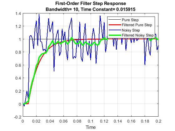
Modify Low_Pass_Filter_Step.m as follows:

a. Change the input to a sine wave with this code:

dt = 0.002; % s

t = 0 : dt : 0.4; % s

f1 = 10 % Hz

s0 = sin(2*pi*f1*t);

% Don't set any data to zero

b. Because the sine wave has both positive values, delete this line: ylim([0,1.5]);

c. Change the filter bandwidth from 10 to 20 Hz:

bw = 20 %(Hz) Bandwidth

d. Change the legend to be this:

legend('Pure Since', 'Filtered Pure Sine', 'Noisy Sine','Filtered Noisy Sine')

Answer

One noise realization looks like this:

.
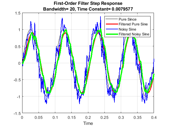