
11.3: Using fzero() to find the intersection of 2 functions
- Page ID
- 88611

\( \newcommand{\vecs}[1]{\overset { \scriptstyle \rightharpoonup} {\mathbf{#1}} } \)
\( \newcommand{\vecd}[1]{\overset{-\!-\!\rightharpoonup}{\vphantom{a}\smash {#1}}} \)
\( \newcommand{\dsum}{\displaystyle\sum\limits} \)
\( \newcommand{\dint}{\displaystyle\int\limits} \)
\( \newcommand{\dlim}{\displaystyle\lim\limits} \)
\( \newcommand{\id}{\mathrm{id}}\) \( \newcommand{\Span}{\mathrm{span}}\)
( \newcommand{\kernel}{\mathrm{null}\,}\) \( \newcommand{\range}{\mathrm{range}\,}\)
\( \newcommand{\RealPart}{\mathrm{Re}}\) \( \newcommand{\ImaginaryPart}{\mathrm{Im}}\)
\( \newcommand{\Argument}{\mathrm{Arg}}\) \( \newcommand{\norm}[1]{\| #1 \|}\)
\( \newcommand{\inner}[2]{\langle #1, #2 \rangle}\)
\( \newcommand{\Span}{\mathrm{span}}\)
\( \newcommand{\id}{\mathrm{id}}\)
\( \newcommand{\Span}{\mathrm{span}}\)
\( \newcommand{\kernel}{\mathrm{null}\,}\)
\( \newcommand{\range}{\mathrm{range}\,}\)
\( \newcommand{\RealPart}{\mathrm{Re}}\)
\( \newcommand{\ImaginaryPart}{\mathrm{Im}}\)
\( \newcommand{\Argument}{\mathrm{Arg}}\)
\( \newcommand{\norm}[1]{\| #1 \|}\)
\( \newcommand{\inner}[2]{\langle #1, #2 \rangle}\)
\( \newcommand{\Span}{\mathrm{span}}\) \( \newcommand{\AA}{\unicode[.8,0]{x212B}}\)
\( \newcommand{\vectorA}[1]{\vec{#1}} % arrow\)
\( \newcommand{\vectorAt}[1]{\vec{\text{#1}}} % arrow\)
\( \newcommand{\vectorB}[1]{\overset { \scriptstyle \rightharpoonup} {\mathbf{#1}} } \)
\( \newcommand{\vectorC}[1]{\textbf{#1}} \)
\( \newcommand{\vectorD}[1]{\overrightarrow{#1}} \)
\( \newcommand{\vectorDt}[1]{\overrightarrow{\text{#1}}} \)
\( \newcommand{\vectE}[1]{\overset{-\!-\!\rightharpoonup}{\vphantom{a}\smash{\mathbf {#1}}}} \)
\( \newcommand{\vecs}[1]{\overset { \scriptstyle \rightharpoonup} {\mathbf{#1}} } \)
\(\newcommand{\longvect}{\overrightarrow}\)
\( \newcommand{\vecd}[1]{\overset{-\!-\!\rightharpoonup}{\vphantom{a}\smash {#1}}} \)
\(\newcommand{\avec}{\mathbf a}\) \(\newcommand{\bvec}{\mathbf b}\) \(\newcommand{\cvec}{\mathbf c}\) \(\newcommand{\dvec}{\mathbf d}\) \(\newcommand{\dtil}{\widetilde{\mathbf d}}\) \(\newcommand{\evec}{\mathbf e}\) \(\newcommand{\fvec}{\mathbf f}\) \(\newcommand{\nvec}{\mathbf n}\) \(\newcommand{\pvec}{\mathbf p}\) \(\newcommand{\qvec}{\mathbf q}\) \(\newcommand{\svec}{\mathbf s}\) \(\newcommand{\tvec}{\mathbf t}\) \(\newcommand{\uvec}{\mathbf u}\) \(\newcommand{\vvec}{\mathbf v}\) \(\newcommand{\wvec}{\mathbf w}\) \(\newcommand{\xvec}{\mathbf x}\) \(\newcommand{\yvec}{\mathbf y}\) \(\newcommand{\zvec}{\mathbf z}\) \(\newcommand{\rvec}{\mathbf r}\) \(\newcommand{\mvec}{\mathbf m}\) \(\newcommand{\zerovec}{\mathbf 0}\) \(\newcommand{\onevec}{\mathbf 1}\) \(\newcommand{\real}{\mathbb R}\) \(\newcommand{\twovec}[2]{\left[\begin{array}{r}#1 \\ #2 \end{array}\right]}\) \(\newcommand{\ctwovec}[2]{\left[\begin{array}{c}#1 \\ #2 \end{array}\right]}\) \(\newcommand{\threevec}[3]{\left[\begin{array}{r}#1 \\ #2 \\ #3 \end{array}\right]}\) \(\newcommand{\cthreevec}[3]{\left[\begin{array}{c}#1 \\ #2 \\ #3 \end{array}\right]}\) \(\newcommand{\fourvec}[4]{\left[\begin{array}{r}#1 \\ #2 \\ #3 \\ #4 \end{array}\right]}\) \(\newcommand{\cfourvec}[4]{\left[\begin{array}{c}#1 \\ #2 \\ #3 \\ #4 \end{array}\right]}\) \(\newcommand{\fivevec}[5]{\left[\begin{array}{r}#1 \\ #2 \\ #3 \\ #4 \\ #5 \\ \end{array}\right]}\) \(\newcommand{\cfivevec}[5]{\left[\begin{array}{c}#1 \\ #2 \\ #3 \\ #4 \\ #5 \\ \end{array}\right]}\) \(\newcommand{\mattwo}[4]{\left[\begin{array}{rr}#1 \amp #2 \\ #3 \amp #4 \\ \end{array}\right]}\) \(\newcommand{\laspan}[1]{\text{Span}\{#1\}}\) \(\newcommand{\bcal}{\cal B}\) \(\newcommand{\ccal}{\cal C}\) \(\newcommand{\scal}{\cal S}\) \(\newcommand{\wcal}{\cal W}\) \(\newcommand{\ecal}{\cal E}\) \(\newcommand{\coords}[2]{\left\{#1\right\}_{#2}}\) \(\newcommand{\gray}[1]{\color{gray}{#1}}\) \(\newcommand{\lgray}[1]{\color{lightgray}{#1}}\) \(\newcommand{\rank}{\operatorname{rank}}\) \(\newcommand{\row}{\text{Row}}\) \(\newcommand{\col}{\text{Col}}\) \(\renewcommand{\row}{\text{Row}}\) \(\newcommand{\nul}{\text{Nul}}\) \(\newcommand{\var}{\text{Var}}\) \(\newcommand{\corr}{\text{corr}}\) \(\newcommand{\len}[1]{\left|#1\right|}\) \(\newcommand{\bbar}{\overline{\bvec}}\) \(\newcommand{\bhat}{\widehat{\bvec}}\) \(\newcommand{\bperp}{\bvec^\perp}\) \(\newcommand{\xhat}{\widehat{\xvec}}\) \(\newcommand{\vhat}{\widehat{\vvec}}\) \(\newcommand{\uhat}{\widehat{\uvec}}\) \(\newcommand{\what}{\widehat{\wvec}}\) \(\newcommand{\Sighat}{\widehat{\Sigma}}\) \(\newcommand{\lt}{<}\) \(\newcommand{\gt}{>}\) \(\newcommand{\amp}{&}\) \(\definecolor{fillinmathshade}{gray}{0.9}\)Using fzero() to find the intersection of 2 functions
Assume you have functions y1(x) and y2(x). Create a new function y3(x) = y1(x) - y2(x). The zero of y3(x) is the intersection of y1(x) and y2(x).
We will have 4 files. A test script file, and 3 function files: function files for each of the 2 functions and a function file that computes the difference of the 2 functions.
% A1. Create a file for a function that computes this straight line:
function y1 = fcn_line_03x(x)

    y1 = 0.3*x;

end
% A2. Create a file for a function that computes this cosine function:
function y2 = cos2x(x);

    y2 = cos(2*x);

end
B. Create a function that computes the difference of these 2 functions:
function y3 = fcn_line_cos_diff(x)

    y3 = fcn_line_03x(x) - cos(2*x);

end
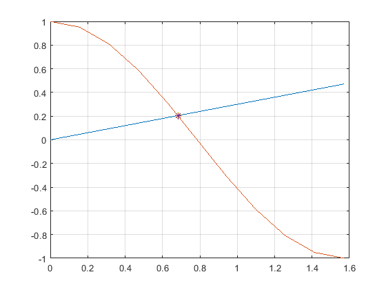
C. The test script m-file call the 2 functions in parts A1 and A2, opens a new figure, and plots the 2 functions:
x = (0: 0.02: 0.5)*pi;

y1 = fcn_line_03x(x);

y2 = cos(2*x);

figure(1)

plot(x,y1)

hold on;

plot(x,y2,'-s')

grid on;

axis equal
% We can see that one intersection of these functions is near x = 0.7 and y = 0.2

D. At the intersection point, y1(x) = y2(x). Rearranging, we get y1(x)- y2(x) = 0.
Create a function file that computes the difference between the 2 functions.
function y3 = fcn_line_cos_diff(x)

    y3 = fcn_line_03x(x) - cos(2*x);

end
So, were can use fzero() to find the point where the difference of the 2 functions is zero.
The code in the test script is:
x_solution = fzero(@fcn_line_cos_diff, 0.7) % near 0.7
% 0.6823
% Verify that this is a solution:
% Verify that this is a solution
y1b = fcn_line_03x(x_solution) % 1st function
% 0.2047
y2b = cos2x(x_solution) % 2nd function
% 0.2047
%% Plot the solution point on the 1st figure
figure(1)

hold on;
plot(x_solution,y1b,'bo','Markersize', 10)

plot(x_solution,y2b,'c*','Markersize', 10)
Add exercises text here.
- Answer
-
Add texts here. Do not delete this text first.
Solution
Add example text here.
.
Intersection of quadratic and cubic functions
A. (2 pts) Create these 2 function files:
y_fun_x2(x)

   y_x2 = x.^2 -4;
end
function y_x3 = y_fun_x3(x)

   y_x3 = x.^3 - 6*x;

end
B1. (2 pt) Begin a script m-file named fzero_y_fun_x2_x3_YourName.m that will plot these functions and will solve for one of their intersections.
At the top of this script, include this code:
clear all; clear functions; close all; format compact; clc;
B2a. (1 pt) Create an x vector from -3 to 3
Choose an increment for x = 0.3, so that the plot will be smooth.
B2b. (2 pts) Use this x vector to compute the corresponding values of y for each of the 2 functions.
y2 = y_fun_x2(x);

y3 = y_fun_x3(x);
B3. (2 pts) Open a figure and plot y2, add "hold on;", the plot y3 on the figure. You will see that they intersect at 3 places.
C1. (2 pts) fzero() finds a root of a single function, so create a 3rd function that computes the difference of the 1st 2 functions:
function y23 = y_2_3_fun(x)

   y23 = y_fun_x2(x) - y_fun_x3(x);

end
Use the x vector to compute values of y for the difference function:
y23 = y_2_3_fun(x)
C2. (1 pt) Open a 2nd figure and plot(x, y23)
D. (6 pts) Use the fzero() function to find a solution where y_2_3_fun(x) = 0.
Use the function handle, @y_2_3_fun as the 1st input of fzero().
For the initial value of x, choose an integer value (whole number) near any one of the intersection points. (Do not use a decimal value that is not an integer.)
- Answer
-
Add texts here. Do not delete this text first.
.
fzero_exp
A. Set
x = (0 : 0.05 : 1)
B. Compute these 2 functions:
y1 = 0.7x
y2 = exp(-2*x)
C. Open a new figure and plot these 2 functions on it.
plot(x,y1)
hold on;
plot(x,y2)
The intersection of these 2 functions is the solution of this transcendental equation:
y1 = y2 or, equivalently, y1 - y2 = 0
D. Find the value of x near 0.5 that is a solution of this equation using the fzero() function as follows:
D1. Rewrite it in the form: fexp(x) = exp(-2*x) - 0.7*x, then create a function file called fexp.m that computes this.
D2. Solve it using the fzero() function, using @fexp as the function handle.
- Answer
-
Add texts here. Do not delete this text first.
.