
11.2: fzero() Examples and Exercises
- Page ID
- 87912

\( \newcommand{\vecs}[1]{\overset { \scriptstyle \rightharpoonup} {\mathbf{#1}} } \)
\( \newcommand{\vecd}[1]{\overset{-\!-\!\rightharpoonup}{\vphantom{a}\smash {#1}}} \)
\( \newcommand{\id}{\mathrm{id}}\) \( \newcommand{\Span}{\mathrm{span}}\)
( \newcommand{\kernel}{\mathrm{null}\,}\) \( \newcommand{\range}{\mathrm{range}\,}\)
\( \newcommand{\RealPart}{\mathrm{Re}}\) \( \newcommand{\ImaginaryPart}{\mathrm{Im}}\)
\( \newcommand{\Argument}{\mathrm{Arg}}\) \( \newcommand{\norm}[1]{\| #1 \|}\)
\( \newcommand{\inner}[2]{\langle #1, #2 \rangle}\)
\( \newcommand{\Span}{\mathrm{span}}\)
\( \newcommand{\id}{\mathrm{id}}\)
\( \newcommand{\Span}{\mathrm{span}}\)
\( \newcommand{\kernel}{\mathrm{null}\,}\)
\( \newcommand{\range}{\mathrm{range}\,}\)
\( \newcommand{\RealPart}{\mathrm{Re}}\)
\( \newcommand{\ImaginaryPart}{\mathrm{Im}}\)
\( \newcommand{\Argument}{\mathrm{Arg}}\)
\( \newcommand{\norm}[1]{\| #1 \|}\)
\( \newcommand{\inner}[2]{\langle #1, #2 \rangle}\)
\( \newcommand{\Span}{\mathrm{span}}\) \( \newcommand{\AA}{\unicode[.8,0]{x212B}}\)
\( \newcommand{\vectorA}[1]{\vec{#1}} % arrow\)
\( \newcommand{\vectorAt}[1]{\vec{\text{#1}}} % arrow\)
\( \newcommand{\vectorB}[1]{\overset { \scriptstyle \rightharpoonup} {\mathbf{#1}} } \)
\( \newcommand{\vectorC}[1]{\textbf{#1}} \)
\( \newcommand{\vectorD}[1]{\overrightarrow{#1}} \)
\( \newcommand{\vectorDt}[1]{\overrightarrow{\text{#1}}} \)
\( \newcommand{\vectE}[1]{\overset{-\!-\!\rightharpoonup}{\vphantom{a}\smash{\mathbf {#1}}}} \)
\( \newcommand{\vecs}[1]{\overset { \scriptstyle \rightharpoonup} {\mathbf{#1}} } \)
\( \newcommand{\vecd}[1]{\overset{-\!-\!\rightharpoonup}{\vphantom{a}\smash {#1}}} \)
\(\newcommand{\avec}{\mathbf a}\) \(\newcommand{\bvec}{\mathbf b}\) \(\newcommand{\cvec}{\mathbf c}\) \(\newcommand{\dvec}{\mathbf d}\) \(\newcommand{\dtil}{\widetilde{\mathbf d}}\) \(\newcommand{\evec}{\mathbf e}\) \(\newcommand{\fvec}{\mathbf f}\) \(\newcommand{\nvec}{\mathbf n}\) \(\newcommand{\pvec}{\mathbf p}\) \(\newcommand{\qvec}{\mathbf q}\) \(\newcommand{\svec}{\mathbf s}\) \(\newcommand{\tvec}{\mathbf t}\) \(\newcommand{\uvec}{\mathbf u}\) \(\newcommand{\vvec}{\mathbf v}\) \(\newcommand{\wvec}{\mathbf w}\) \(\newcommand{\xvec}{\mathbf x}\) \(\newcommand{\yvec}{\mathbf y}\) \(\newcommand{\zvec}{\mathbf z}\) \(\newcommand{\rvec}{\mathbf r}\) \(\newcommand{\mvec}{\mathbf m}\) \(\newcommand{\zerovec}{\mathbf 0}\) \(\newcommand{\onevec}{\mathbf 1}\) \(\newcommand{\real}{\mathbb R}\) \(\newcommand{\twovec}[2]{\left[\begin{array}{r}#1 \\ #2 \end{array}\right]}\) \(\newcommand{\ctwovec}[2]{\left[\begin{array}{c}#1 \\ #2 \end{array}\right]}\) \(\newcommand{\threevec}[3]{\left[\begin{array}{r}#1 \\ #2 \\ #3 \end{array}\right]}\) \(\newcommand{\cthreevec}[3]{\left[\begin{array}{c}#1 \\ #2 \\ #3 \end{array}\right]}\) \(\newcommand{\fourvec}[4]{\left[\begin{array}{r}#1 \\ #2 \\ #3 \\ #4 \end{array}\right]}\) \(\newcommand{\cfourvec}[4]{\left[\begin{array}{c}#1 \\ #2 \\ #3 \\ #4 \end{array}\right]}\) \(\newcommand{\fivevec}[5]{\left[\begin{array}{r}#1 \\ #2 \\ #3 \\ #4 \\ #5 \\ \end{array}\right]}\) \(\newcommand{\cfivevec}[5]{\left[\begin{array}{c}#1 \\ #2 \\ #3 \\ #4 \\ #5 \\ \end{array}\right]}\) \(\newcommand{\mattwo}[4]{\left[\begin{array}{rr}#1 \amp #2 \\ #3 \amp #4 \\ \end{array}\right]}\) \(\newcommand{\laspan}[1]{\text{Span}\{#1\}}\) \(\newcommand{\bcal}{\cal B}\) \(\newcommand{\ccal}{\cal C}\) \(\newcommand{\scal}{\cal S}\) \(\newcommand{\wcal}{\cal W}\) \(\newcommand{\ecal}{\cal E}\) \(\newcommand{\coords}[2]{\left\{#1\right\}_{#2}}\) \(\newcommand{\gray}[1]{\color{gray}{#1}}\) \(\newcommand{\lgray}[1]{\color{lightgray}{#1}}\) \(\newcommand{\rank}{\operatorname{rank}}\) \(\newcommand{\row}{\text{Row}}\) \(\newcommand{\col}{\text{Col}}\) \(\renewcommand{\row}{\text{Row}}\) \(\newcommand{\nul}{\text{Nul}}\) \(\newcommand{\var}{\text{Var}}\) \(\newcommand{\corr}{\text{corr}}\) \(\newcommand{\len}[1]{\left|#1\right|}\) \(\newcommand{\bbar}{\overline{\bvec}}\) \(\newcommand{\bhat}{\widehat{\bvec}}\) \(\newcommand{\bperp}{\bvec^\perp}\) \(\newcommand{\xhat}{\widehat{\xvec}}\) \(\newcommand{\vhat}{\widehat{\vvec}}\) \(\newcommand{\uhat}{\widehat{\uvec}}\) \(\newcommand{\what}{\widehat{\wvec}}\) \(\newcommand{\Sighat}{\widehat{\Sigma}}\) \(\newcommand{\lt}{<}\) \(\newcommand{\gt}{>}\) \(\newcommand{\amp}{&}\) \(\definecolor{fillinmathshade}{gray}{0.9}\)fzero() is a "function of a function", because it needs a "handle" to a function that defines the equation whose root it will find. fzero() can be used either to find a zero of a single functions and or to find the intersection point of 2 functions.
Using fzero() to find the root of a single function
The way it works is as follows: It finds an interval containing the initial point. It uses nearby points to approximate derivatives and estimate where the zero is. It then re-evaluates the function at this new x value. It repeats this procedure until it finds a point where the function is zero or very nearly zero.
Find a root of a 5th-order polynomial:
We will find a root of this 5th-order polynomial:
y = x.^5 - 4*x.^2 -10*x + 1;
Method 1: A straightforward way to do this is to create a function file for this:
% fpoly5.m:
function y = fpoly5(x)
y = x.^5 - 4*x.^2 -10*x + 1;
end
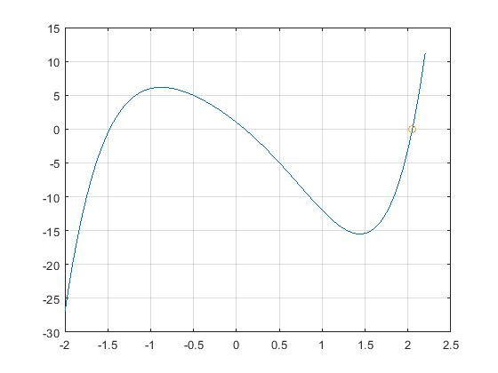
Create a separate m-file script (fzero_poly5.m) to visualize this function and to estimate the root.
%% A. Open a new figure and plot the function
x = -2:0.05:2.2;
y = fpoly5(x);
figure
plot(x,y)
grid on;
%% B. the value of x near x=2.1 that makes y = 0
x_solution = fzero(@fpoly5, 2.1) % @fpoly5 is a function "handle" to the file fpoly5.m
% fzero() evaluates the function fpoly5(x) multiple times, until it converges to a root. (A root is a value that makes the function = 0)
% x_solution = 2.0517
% Verify that this is a solution:
yb = fpoly5(x_solution)
% 7.1054e-15
hold on;
plot(x_solution,yb,'o')
----
Method 2: Another way is to create a local sub-function at the bottom of the m-file script. This method currently works in MATLAB, but not Octave.
Solution
.
%% A. Create this function
function y1 = y_fun1(x)
y1 = log(x)./x.^2 -0.1;
end
Create a separate m-file script to visualize this function and to estimate the root.
%% B. (1 pt) In this 2nd file, create an x vector from 0.2 to 2.0
% Choose an increment for x, such that the plot will be smooth--that is, no visible straight lines.
x = 1: 0.1 :6;
% (1 pt) Evaluate the equation using your x vector
y1 = y_fun1(x);
%% C. (1 pt) Open figure and plot this function.
% A plot of the function lets us estimate a root.
figure(1)
plot(x,y1)
grid on;
title('fzero1root\_fcnfile\_example.m CSmith')
hold on;
plot(x,zeros(size(x)),'r') % Plot a line for y = 0
%% D. (4 pts) Use the fzero() function to find a root near x = 4
Solution
x_solution = fzero(@y_fun1, 4)
% @y_fun1 = "function handle" to y_fun1.m
% The function y_fun1(x) must have a single input variable.
% fzero chooses the values of x for computing the function
% x_solution = 3.5656
%% E. fzero() can also be used to find a root between 2 values
x_solution = fzero(@y_fun1, [3,5])
.
fzero for y = log10(x) + 0.44;
%% Create a function m-file that computes y = log10(x) + 0.44;
% Set
x = 0 : 0.02 : 1;
Create a separate m-file script to visualize this function and to estimate the root.
% Compute y for this x vector using your function.
% Open a figure and plot(x, y)
% Turn the grid on
% Use fzero() to find a root near 0.4 of this function
- Answer
-
Add texts here. Do not delete this text first.
.