19.5.1: ODE45 Examples and Exercises

If you have taken a differential equations course, then you learned techniques to solve a variety of differential equations analytically.
Other ODE's cannot be solved analytically. They can only be solved numerically.

ode45() requires a differential equation function to be coded in a particular format. This function can be implemented in 3 ways in MATLAB and 2 ways in Octave.

1. The ODE function can be a coded as its own file. This is straight-forward. It works in both MATLAB and Octave. It is illustrated in the 2nd example.
2. An "anonymous function" (an in-line function). It can be used when the function is a single line of code. This can work for a 1st order ode, but not easily for a 2nd order ode. using an An anonymous function is not illustrated here.
3. The ODE function can be placed at the bottom of the script file. This is called a subfunction. It works in MATLAB, but not in the current version of Octave. (However Octave allows a subfunction within a function file, but not in a script file.) It is illustrated in the 1st example.
4. The simplest way to use ODE45() is specify 3 general parameters in the argument list and put the function specific parameters in the function file or anonymous specification. The general parameters are:
   1. The function handle
   2. The time interval
   3. The initial vector of x and its derivatives.
5. The function specific parameters can be specified in the function call, as shown in the last example below. This takes more care to be done correctly.

In previous chapters in this book, we have generally used separate files for functions used by MATLAB functions such as fzero() and integral(). I recommend creating a separate file for function that could be used multiple times with different inputs; this is a general purpose function. However, for the ode() function, the user codes a function with specific parameters defined within the function (not general purpose), so it makes sense to define it as a subfunction at the bottom of the script file (if you are using MATLAB).

The 1st example of using the ode45() function is a 1st order ODE; it can be easily solved analytically. The example solves it with ode45(); the solution can be verified vs. the analytical solution.

The 2nd example of using the ode45() function is a 2nd order ODE; it can be solved analytically only with difficulty.

Example \(\PageIndex{1}\) ODE of a Parabola

This example if of a parabola as a function of time. The code for this example illustrates using a sub-function within the test file.

The equation equation for this parabola is 

y(t) = 2*t^2 - 0.5

% dydt_4t_ODE_example.m
% This example uses a sub-function within the test file.
% The equation equation for this parabola is y(t) = 2*t^2 -4

% The syntax of ode45 is:
% [T_OUT, Y_OUT] = ode45(@ODEFUN, TSPAN, Y0)
% @ODEFUN is the handle to the ode function.
TSPAN = [-1.0, 1.0]; % s
% TSPAN is a 2-element vector = [T0, TFINAL]
% specifying the time interval
Y0 = 1.5; % the initial value of y(t)
[tout, yout] = ode45(@dy4_ODE, TSPAN, Y0);
% Note: Instead of the user specifying a time vector,
% ode45 computes a time vector with appropriate time increments.

% Plot the function computed by ode45
figure;
plot(tout, yout, '-o')
title('ode45() for dy/dt = 4t')
grid on;

function dydt = dy4_ODE(t,y)
dydt = 4*t;
end

The plot is shown in the solution.

Solution

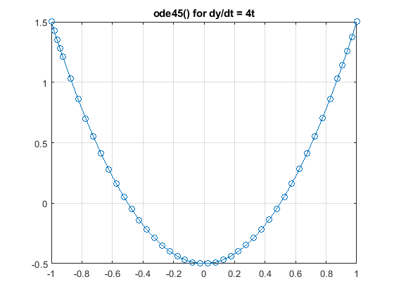
A plot of the solution.

 

 

 

 

 

 

 

.

Example \(\PageIndex{2}\) Damped spring example

This example uses a separate function file.

The 2nd-order differential equation for an under-damped spring oscillator is:

\(m \frac{d^2 x}{dt^2} + c \frac{dx}{dt} + kx = 0\)

The constants for this example are:

m = 2
c = 0.4
k = 4

The differential equation and the constants are defined in the function file "ODE_Damped_Spring.m"

For a 2nd order differential equation, ODE45 requires that the function file has a column vector of 2 inputs and a column vector of 2 outputs.

The input vector, x, has the position and it's 1st derivative:

x(1) = x = the position
x(2) = dx/dt = the 1st derivative of x(1)

The output vector is the derivative of the input vector:

xdot(1) = dx/dt

xdot(2) = d^2x/dt^2 = the derivative of dx/dt

\(\frac{d^2 x}{dt^2} = -\frac{1}{m} (c \frac{dx}{dt} + kx) \)

The code for the function is given here and is also attached as ODE_Damped_Spring.m

function xdot = ODE_Damped_Spring(t, x)
% This models the oscillation of a damped spring
% Inputs:
% t = time is not used, since this is a time-independent model
% x = a column vector with 2 elements:
% x(1) = x = the position
% x(2) = dx/dt = the 1st derivative of x
% Output
% xdot = a column vector with 2 elements:
% xdot(1) = 1st derivative of x = x(2)
% xdot(2) = 2nd derivative of x from this equation:
% m(d^2x/dt^2) + c(dx/dt) + kx = 0
% Constants of the equations
m = 2;
c = 0.4;
k = 4;
xdot = zeros(2,1); % Initialize the output
xdot(1) = x(2); % 1st derivative
xdot(2) = -(1/m)*(c*x(2) + k*x(1)); % 2nd derivative

The test program sets the "initial conditions" (the starting position and derivative), calls ODE45 with a handle to the diferential equation function, and plots the result. This is given here and is also attached as ODE_Damped_Spring_test.m.

%% ODE_Damped_Spring_test
% m(d^2x/dt^2) + c(dx/dt) + kx = 0
% m = 2;
% c = 0.4;
% k = 4;
% To compute the solution to this equation,
% we need a function: ODE_Damped_Spring.m
% The x input needs to be a column vector.
x0 = [10;  % Initial values of x
       0]; % Initial values the 1st derivative x
Time_Span = [0, 40.0]; % (s)
[t_ex2, x_ex2] = ode45(@ODE_Damped_Spring, Time_Span, x0);

figure;
plot(t_ex2, x_ex2(:,1), 'o-')
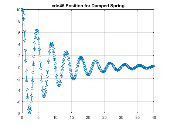
title('ode45 Position for Damped Spring')
grid on;

The resulting plot is shown in the solution.

Solution

The resulting plot is shown here.

 

.

Example \(\PageIndex{2}\) Passing function parameters thru the ODE45 call

This is the differential equation function file is shown here. Note that in addition to the required x and t inputs, it has 3 function specif parameters: m, c, & 

function dxdt = damped_spring1(t, x, m, c, k)
dxdt = zeros(2, 1);
dxdt(1) = x(2);
dxdt(2) = (-c*x(2) - k*x(1)) / m;
end

The main script that includes the ode45() function call is this:

m = 3;
c= 0.3;
k= 9;

time_span = [0 33];
xx0 = [0; 3];

[t,xx] = ode45(@(t, x) damped_spring1(t, x, m, c, k), time_span, xx0);

figure
plot(t, xx(:,1))
title ('x(t) - Position vs Time')
xlabel('Time (s)')
ylabel('x(t)')

figure
plot(t, xx(:,2))
title('dx/dt = Velocity vs Time')
xlabel('Time (s)')
ylabel('dx/dt')

In the standard form of calling ode45(), one does not need to specify t and x.

But in this advanced form, t and x need to be specified, followed by the function-specific parameters:

[t,xx] = ode45(@(t, x) damped_spring1(t, x, m, c, k), time_span, xx0);

Solution

 

 

.

Exercise \(\PageIndex{1}\) Logistic ODE Equation Assignment

Background:

The Logistic ODE equation is:

dP/dt = r*P*(1 - P/K)

where:

P = population

r = growth rate when the population is small
K = carrying capacity (max. value of P)

This a modification of the version of the exponential population growth ODE which assumes that the population is changing at a constant rate.

When the population population is small, P/K is small, then dP/dt is approximately = r*P. This means that the growth rate is proportional to the population and P grows exponentially.

When the population population becomes close to K, then P/K is near 1, so dP/dt is approximately = 0 and P is approximately constant.

Assignment:

Create an m-file script that computes the solution to the logistic differential equation.

Start with this line:

clear all; close all; clc; format compact

(1 pt) Set these parameters:

tspan = [1,100] % [timeBegin, timeEnd] = the time span for the computation.

P0 = 10 % Initial population

(5 pts) Write the 1 line of code that calls the ode45() solver function with its 3 inputs:

@dPdt (the function handle), tspan, and P0

The outputs are [t, P]

(2 pts) Open a figure and plot P vs. t with this code:

figure;
plot(t, P);
title('Logistic Equation')
xlabel('time')
ylabel('Population')
grid on;

(2 pts) Put the following code that computes the derivative of P as a local function at the bottom of your m-file:

%% Local function
% Ordinary Differential Equation
function dPdt = logistic_ode(t, P)
r = 0.065; % growth rate
K = 38; % max value of P
dPdt = r*P*(1 - P/K);
end

If you want to learn more about the Logistic ODE, visit these links:

https://mathworld.wolfram.com/LogisticEquation.html (Links to an external site.)
https://www.matlab-monkey.com/ODE/logisticV1/logisticV1Pub.html (Links to an external site.)

Answer

The solution is not given here. Your plot should show the population increasing until it gets near to the maximum value, K, then the curve becomes nearly horizontal.

.