11.1: Compression buckling of thin rectangular plates

Last updated
Save as PDF

Page ID: 95322

$ \newcommand{\vecs}[1]{\overset { \scriptstyle \rightharpoonup} {\mathbf{#1}} } $

$ \newcommand{\vecd}[1]{\overset{-\!-\!\rightharpoonup}{\vphantom{a}\smash {#1}}} $

$ \newcommand{\id}{\mathrm{id}}$ $ \newcommand{\Span}{\mathrm{span}}$

( \newcommand{\kernel}{\mathrm{null}\,}\) $ \newcommand{\range}{\mathrm{range}\,}$

$ \newcommand{\RealPart}{\mathrm{Re}}$ $ \newcommand{\ImaginaryPart}{\mathrm{Im}}$

$ \newcommand{\Argument}{\mathrm{Arg}}$ $ \newcommand{\norm}[1]{\| #1 \|}$

$ \newcommand{\inner}[2]{\langle #1, #2 \rangle}$

$ \newcommand{\Span}{\mathrm{span}}$

$ \newcommand{\id}{\mathrm{id}}$

$ \newcommand{\Span}{\mathrm{span}}$

$ \newcommand{\kernel}{\mathrm{null}\,}$

$ \newcommand{\range}{\mathrm{range}\,}$

$ \newcommand{\RealPart}{\mathrm{Re}}$

$ \newcommand{\ImaginaryPart}{\mathrm{Im}}$

$ \newcommand{\Argument}{\mathrm{Arg}}$

$ \newcommand{\norm}[1]{\| #1 \|}$

$ \newcommand{\inner}[2]{\langle #1, #2 \rangle}$

$ \newcommand{\Span}{\mathrm{span}}$ $ \newcommand{\AA}{\unicode[.8,0]{x212B}}$

$ \newcommand{\vectorA}[1]{\vec{#1}} % arrow$

$ \newcommand{\vectorAt}[1]{\vec{\text{#1}}} % arrow$

$ \newcommand{\vectorB}[1]{\overset { \scriptstyle \rightharpoonup} {\mathbf{#1}} } $

$ \newcommand{\vectorC}[1]{\textbf{#1}} $

$ \newcommand{\vectorD}[1]{\overrightarrow{#1}} $

$ \newcommand{\vectorDt}[1]{\overrightarrow{\text{#1}}} $

$ \newcommand{\vectE}[1]{\overset{-\!-\!\rightharpoonup}{\vphantom{a}\smash{\mathbf {#1}}}} $

$ \newcommand{\vecs}[1]{\overset { \scriptstyle \rightharpoonup} {\mathbf{#1}} } $

$ \newcommand{\vecd}[1]{\overset{-\!-\!\rightharpoonup}{\vphantom{a}\smash {#1}}} $

11.7 Compression buckling of thin rectangular plates

Consider the perfectly flat plate subject to a longitudinal compressive force of magnitude P_x applied in a spatially uniform manner along edges x = 0 and x = a, as shown in figure 11.24. The equilibrium response of the plate in linear theory is that of pure compression in the x-y plane with no out-of-plane deflection of the midsurface. That is, in the pre-buckling equilibrium state the plate remains flat. The normal stress σ_x in the plate is spatially uniform, and we write it as $σ_{x} = - σ$ $math-2704.png$ , where $σ = P_{x} / (b t)$ $math-2705.png$ is the applied compressive stress.

At a critical value of the compressive force P_xcr the plate will buckle, or deflect out of the flat pre-buckling equilibrium state. To determine this critical force we have to consider a slightly deflected equilibrium configuration of the plate, similar to the analysis of the perfect column presented in article 11.1. Refer to Brush and Almroth (1975) for the details of this adjacent equilibrium analysis for the critical force.

A flat rectangular plate of width a and height b is placed under a uniformly distributed compressive axial load cap P sub x along the lengthwise x axis. Y is shown to be along the height, and denotes the origin is at the bottom left corner of the plate. The plate is shown to be of thickness t, and is pinned at each along the x axis. The z axis is aligned with thickness, and shows the origin to be at the left pinned edge. — Fig. 11.24 Uniformly applied compressive forces applied to opposite longitudinal edges of a rectangular plate.

Instead of a detailed adjacent equilibrium analysis of the plate, we can make a comparison to the critical force determined for the pinned-pinned column in figure 11.6. The configuration of the plate comparable to the pinned-pinned column has simply supported, or hinged, edges at x = 0 and x = a, and has free edges at y = 0 and y = b. The compressively loaded plate for these boundary conditions is called a wide column. The critical force for the pinned-pinned column is

$\begin{align} P_{c r} = π^{2} E I L^{2} . & (11.106) \end{align}$ $math-2706.png$

For the plate, replace the modulus of elasticity E in the column formula by $E / (1 - v^{2})$ $math-2707.png$ , since the plate is stiffer than the column. Also set L = a for the plate. The formula for the second area moment of a rectangular cross section is 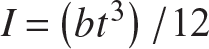$I = (b t^{3}) / 12$ $math-2708.png$ . Hence, eq. (11.106) transforms to

$\begin{align} P_{x c r} = π^{2} (\frac{E}{1 - v^{2}}) (\frac{1}{a^{2}}) (\frac{b t^{3}}{12}) = π^{2} (\frac{E t^{3}}{12 (1 - v^{2})}) \frac{b}{a^{2}} . & (11.107) \end{align}$ $math-2709.png$

For the wide column configuration of the plate, the critical load is written in the form

$\begin{align} P_{x c r} = \frac{π^{2} D b}{a^{2}}, & (11.108) \end{align}$ $math-2710.png$

where the bending stiffness, or flexural rigidity, of the plate is defined as

$\begin{align} D = \frac{E t^{3}}{12 (1 - v^{2})} . & (11.109) \end{align}$ $math-2711.png$

The critical compressive stress at buckling is simply $σ_{c r} = P_{x c r} / (b t)$ $math-2712.png$ . Divide eq. (11.107) by area bt to get

$\begin{array}{l} σ_{c r} = π^{2} (\frac{E t^{3}}{12 (1 - v^{2})}) \frac{b}{a^{2}} \frac{1}{b t} = π^{2} \frac{E}{12 (1 - v^{2})} {(\frac{t}{b})}^{2} {(\frac{b}{a})}^{2} . \end{array}$ $math-2713.png$

By convention, this critical compressive stress is written in the form

$\begin{align} σ_{c r} = k_{c} π^{2} \frac{E}{12 (1 - v^{2})} {(\frac{t}{b})}^{2} & (11.110) \end{align}$ $math-2714.png$

where k_c is a nondimensional buckling coefficient for compressive loading, which is a function of the plate aspect ratio a∕b. For the unloaded edges free and the loaded edges simply supported, this buckling coefficient is

$\begin{align} k_{c} = \frac{1}{{(a / b)}^{2}} wide column . & (11.111) \end{align}$ $math-2715.png$

For other support conditions on the edges x = 0, x = a, y = 0, and y = b, the critical compressive stress is also given by eq. (11.110) but the compressive bucking coefficient is a different function of the plate aspect ratio. The transition from column to plate as supports are added along the unloaded edges (y = 0 and y = b) are depicted in figure 11.25 on page 319. The compressive buckling coefficient is plotted for various support conditions as shown in figure 11.26 on page 320. Note that some of the curves for the buckling coefficient exhibit cusps, or discontinuous slopes, at selected values of the plate aspect ratio. The cusps correspond to changes in the half wave length of the buckle pattern along the x-direction. In particular, for the plate with simple support on all four edges, case C in figure 11.26 on page 320, note that k_c = 4 for integer aspect ratios.

11.7.1 Simply supported rectangular plate

Consider a plate simply supported on all four edges and subject to uniform compressive on edges x = 0 and x = a. In the pre-buckling equilibrium configuration the plate remains flat, $w_{0} (x, y) = 0$ $math-2716.png$ , with a spatially uniform compressive stress equal to the applied compressive stress σ. From the method of adjacent equilibrium, the out-of-plane displacement of the plate at the onset of buckling is

$\begin{align} w_{1} (x, y) = A_{1} sin (\frac{m π x}{a}) sin (\frac{n π y}{b}), & (11.112) \end{align}$ $math-2717.png$

where m and n are positive integers and A₁ is an arbitrary amplitude. Integer m corresponds to the number of half waves in the x-direction and integer n corresponds to the number of half waves in the y-direction. Thus, specific values of integers m and n in eq. (11.112) characterize a buckling mode, and for each buckling mode there is a corresponding buckling stress. Equation (11.110) is the formula for the compressive stress at buckling, with the compressive buckling coefficient given by

$\begin{align} k_{c} = {(\frac{m}{a / b} + n^{2} \frac{(a / b)}{m})}^{2} m, n = 1, 2, \dots . & (11.113) \end{align}$ $math-2718.png$

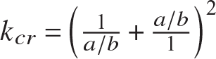
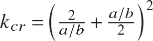
The critical stress is the lowest buckling stress, which occurs for a certain choice of m and n. Since k_c is directly proportional to powers of integer n, the minimum value of k_c occurs for n = 1. Then minimum values of k_c are related to a∕b and integer m by

$\begin{align} k_{c} = {(\frac{m}{a / b} + \frac{(a / b)}{m})}^{2} . & (11.114) \end{align}$ $math-2719.png$

Critical values of the compressive buckling coefficient as a function of a few aspect ratios are listed in table 11.4.

A plate placed under a compressive load along two of its edges. A plate will deform similar to column buckling if these loaded edges are pinned, but the others are left free. If one of the other edges is pinned, the remaining free edge will buckle similar to column buckling. Finally, if all four edges are pinned, the plate will show multiple modes, with the first mode showing across the plate, between the unloaded edges, while a higher move resembling a sinusoidal wave appears between the loaded edges. 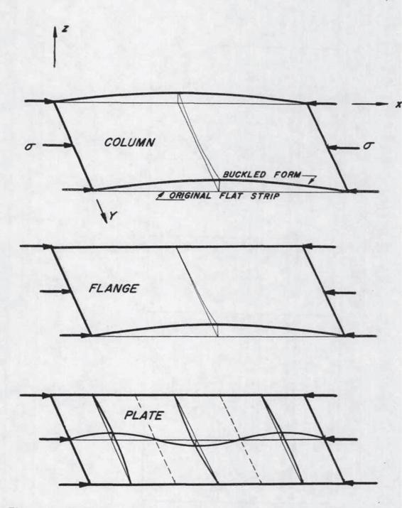— Fig. 11.25 Transition form column to plate as supports are added along unloaded edges. Note changes in buckle configurations (NACA TN 3781, figure 1).

Five plates are shown with varying boundary conditions on the unloaded edges. Cap A is clamped on both edges. Cap B is simply supported on one edge and clamped on the other. Cap C is simply supported on both edges. Cap D is free on one edge and clamped on the other. Cap E is free on one edge and simply supported on the other. The plot shows length a over width b on the horizontal axis, and load factor k sub c on the vertical axis. As width b outpaces length a, higher modes begin to supersede the lower ones, resulting in numerous bumps along each line. However, as the un-loaded edge conditions are made less restrictive, the associated curves decrease and become smoother. — Fig. 11.26 Compression buckling coefficient for flat rectangular plates (NACA TN 3781, figure 14).

Table 11.4 Compression buckling coefficient for selected plate aspect ratios

Plate aspect ratio	Number of half waves in the x-direction	Critical compressive buckling coefficient
$0 < a / b \leq \sqrt{2}$ $math-2720.png$	m = 1	$k_{c r} = {(\frac{1}{a / b} + \frac{a / b}{1})}^{2}$ $math-2721.png$

$\sqrt{2} \leq a / b \leq \sqrt{6}$ $math-2722.png$	m = 2	$k_{c r} = {(\frac{2}{a / b} + \frac{a / b}{2})}^{2}$ $math-2723.png$

$\sqrt{6} \leq a / b \leq \sqrt{12}$ $math-2724.png$	m = 3	$k_{c r} = {(\frac{3}{a / b} + \frac{a / b}{3})}^{2}$ $math-2725.png$

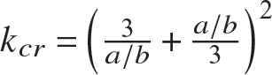
These critical values of the compression buckling coefficient are plotted as case C in figure 11.26 on page 320. The buckling modes for three integer values of the aspect ratio are depicted in figure 11.27. There is one half wave across the width (n = 1) and the number of half waves across the length, m, increases with increasing aspect ratio. For integer values of the aspect ratio the critical value of the compressive buckling coefficient k_cr = 4, and it follows that the critical compressive stress is

$\begin{align} σ_{c r} = 4 π^{2} \frac{E}{12 (1 - v^{2})} {(\frac{t}{b})}^{2} \frac{a}{b} = m = 1, 2, 3, \dots n = 1 . & (11.115) \end{align}$ $math-2726.png$

From eq. (11.112) the length of a half wave in the x-direction is a∕m, and the length of a half wave in the y-direction is the plate width b for n = 1. These half wave lengths are the same when $a / m = b$ $math-2727.png$ , or $a / b = m$ $math-2728.png$ . That is, the half wave lengths in the x- and y-directions are the same for integer values of the aspect ratio. Hence, for integer values of the plate aspect ratio the buckling mode consists of a sequence of square buckles.

A flat plate of length a along the x axis and width b along the y axis is shown to be simply supported on all four sides. For a over b equal to 1, the buckling will show as the plate bulging upward in the center, evenly across the whole plate. With a over b equal to 2, the buckling will resemble two versions of the first mode placed side by side in the x direction, with one being upward and the other downward, forming a sinusoidal curve through the center in the x-direction. Increasing a over b equal to 3, results in a third curvature, now resembling three plates connected along their edges, each buckling in their first mode, to create a longer sinusoidal wave through the center. Node lines are labeled at the points where the plates remain flat at the boundaries of each curvature. 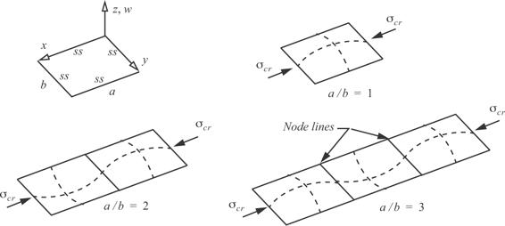— Fig. 11.27 Compression buckling modes for integer aspect ratios of a simply supported rectangular plate.

Example 11.4 Critical load for simply supported rectangular plate in compression

Let a = 20 in., b = 10 in., $t = 0.10$ $math-2729.png$ in., $E = 10 \times 1 0^{6} lb . / in .^{2}$ $math-2730.png$ , and $v = 0.3$ $math-2731.png$ . From eq. (11.110) the critical compressive stress

$\begin{align} σ_{cr} = k_{c} (903.81 lb . / {in.}^{2}) . & (a) \end{align}$ $math-2732.png$

From eq. (11.114) the compression buckling coefficient is

$\begin{align} k_{c} = {(\frac{m}{2} + \frac{2}{m})}^{2} . & (b) \end{align}$ $math-2733.png$

For $m = 1, 2, 3, k_{c} = 6.25, 4.0, 4.694$ $math-2734.png$ , respectively. For larger values of m, coefficient k_c is larger. The minimum value of k_c is 4 corresponding to m = 2. Hence, the critical stress is

$\begin{align} σ_{cr} = 3, 615.24 lb . / {in.}^{2} . & (c) \end{align}$ $math-2735.png$

The critical compressive load P_cr = σ_crbt. Hence,

$\begin{align} P_{cr} = 3, 615 lb. . & (d) \end{align}$ $math-2736.png$

The buckling mode for $(m, n) = (2, 1)$ $math-2737.png$ has one half sine wave in the transverse direction and two half waves in the longitudinal direction. The load $P_{cr} = 3, 615 lb.$ $math-2738.png$ is the lowest load at which such a plate can lose its stability.

■

11.8 Buckling of flat rectangular plates under shear loads

Consider a thin, rectangular plate with a thickness denoted by t, and the in-plane dimensions denoted by a and b, where $0 < t ≪ b \leq a$ $math-2739.png$ . Note that a denotes the long dimension of the plate and b denotes the short dimension. It is subject to uniformly distributed shear stress τ as illustrated in figure 11.28. From Mohr’s circle for plane stress, the state of pure shear is equivalent to tensile and compressive normal stresses at forty-five degrees to the direction of pure shear. It is this compressive normal stress that leads to buckling of the thin plate subjected to shear.

A flat plate of length a along the x axis and height b along the y axis is placed under shear loading tau along each edge. The top and right edged point to the top right corner, while the bottom and left edges point towards the bottom-left corner. — Fig. 11.28 Plate subject to in-plane shear loading.

The critical value of the shear stress per unit length, τ_cr, is given by the formula

$\begin{align} τ_{c r} = k_{s} π^{2} \frac{E}{12 (1 - v^{2})} {(\frac{t}{b})}^{2}, & (11.116) \end{align}$ $math-2740.png$

where k_s is a nondimensional buckling coefficient for shear loading. This buckling coefficient is a function of the plate aspect ratio a∕b and the boundary conditions applied to the plate. Values of the shear buckling coefficient are given in figure 11.30 on page 324. The buckling mode labeled the symmetric mode in the figure pertains to a buckled form that is symmetric with respect to a diagonal across the plate at the node line slope. For a narrow range of aspect ratios the plate buckles in an antisymmetric mode. For an infinitely long strip, or a∕b→∞, $k_{s} = 5.35$ $math-2741.png$ for simply supported, or hinged, edges at $y = 0, b$ $math-2742.png$ , and $k_{s} = 8.98$ $math-2743.png$ for clamped edges.

A least squares fit of the shear buckling coefficient as a function of the plate aspect ratio is convenient in problem solving. For the simply supported plate, or the plate with hinged edges, the data listed in table 11.5 was read from the graph in figure 11.30.

Table 11.5 Shear buckling coefficient for selected plate aspect ratios

*a/b*	$k_{s}$ $math-2744.png$
1	9.6
2	6.4
3	5.8
4	5.7
5	5.5

These data are fit to the functions 1 and $\frac{1}{a / b}$ $math-2745.png$ . The result of the least squares fit to these data is

$\begin{align} k_{s} = 4.22565 + \frac{5.19931}{a / b} 1 \leq a / b \leq 5 . & (11.117) \end{align}$ $math-2746.png$

The least squares fit and the input data are plotted in figure 11.29.

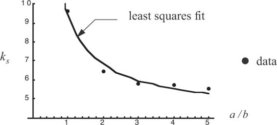
A plot shows a over b on the horizontal axis and load factor k sub s on the vertical axis. The least squares fit line passes through the experimental results and appears to match the general trend of the points, asymptotically approaching a k sub s value of 5. — Fig. 11.29 Graph of eq. (11.117) compared to discrete data listed in table 11.5.

Experimental results show two lines on a plot with a over b on the horizontal axis and k sub s on the vertical axis. Both lines begin at a over b equal 1 one and move through a value of 5. The lower line begins at approximately k sub s equal 10, gradually decreasing to asymptotically approach k sub s equal to 5. The upper line begins at approximately 15, and asymptotically approaches k sub s equal to 9 in a similar fashion. The first decreasing portions are labeled as symmetric modes. The points where each begins to level off is denoted as antisymmetric modes. The final relatively level portion is denoted as symmetric modes again. The upper line represents clamped edges, while the lower line represents hinged or simply supported edges. — Fig. 11.30 Shear-buckling-stress coefficient of plates as a function of a/b for clamped and hinged edges (NACA TN 3781, figure 22).

11.9 Buckling of flat rectangular plates under combined compression and shear

A plate subject to uniformly applied longitudinal compression and shear is shown in figure 11.31. The critical combination of shear and compression stresses under different boundary conditions and different aspect ratios of the plate can be approximated to a sufficient accuracy by

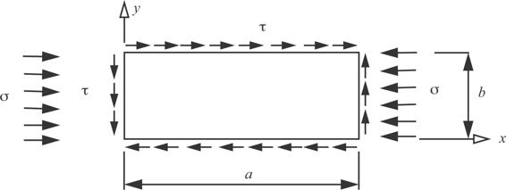
A rectangular plate is now shown with both the shear and normal loading of previous figures, with compressive sigmas on each end and shear tau pointing towards the top right and bottom left corners. — Fig. 11.31 Plate subject to longitudinal compression and in-plane shear loading.

$\begin{align} {(\frac{τ}{τ_{cr}})}^{2} + (\frac{σ}{σ_{cr}}) = 1, & (11.118) \end{align}$ $math-2747.png$

where $τ_{cr}$ $math-2748.png$ and $σ_{cr}$ $math-2749.png$ are the critical values of the separately acting shear stress and the compression normal stress, respectively (NACA TN 3781, pp. 38, 39). Equation (11.118) is plotted in figure 11.32.

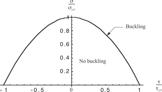
A downward opening parabola is shown on a plot with shear tau over tau sub cr on the horizontal axis and axial sigma over sigma sub cr on the vertical axis. The parabola passes through x-intercepts of plus and minus one, as well as a y-intercept of 1. — Fig. 11.32 Buckling interaction relationship for critical combinations of shear and compression.

Example 11.5 Wing rib spacing based on a buckling constraint

The stringer stiffened box beam that is the main spar in a wing is shown in figure 11.33. For a pull-up maneuver, the calculated transverse shear force $V_{y} = 25, 000 lb$ $math-2750.png$ . and the bending moment $M_{x} = - 4.14 \times 1 0^{6} lb$ $math-2751.png$ –in. at the wing root. The thickness and width of the upper and lower cover skins are $t_{f} = 0.5 in$ $math-2752.png$ . and b_f = 24in., respectively. The thickness and height of the left and right webs are $t_{w} = 0.30 in$ $math-2753.png$ . and $b_{w} = 13 in$ $math-2754.png$ ., respectively, and the flange area of the stringers $A_{f} = 2.0 {in.}^{2}$ $math-2755.png$ . The material is isotropic with properties $E = 10 \times 1 0^{6} lb / {in.}^{2}$ $math-2756.png$ and $v = 0.3$ $math-2757.png$ . For M_x < 0, the upper skin is in compression. Determine the rib spacing, denoted by a, such that the margin of safety for buckling of the upper skin is slightly positive.

The wing box of an airfoil section is represented by a rectangular box formed by the the wing’s skin, the forward and rear spars distance b sub f apart, and the spacing between ribs distance a apart. Four stringers run along the top and bottom edges of the spar faces. The local coordinate frame uses x pointing out of the front of the wing, while y is out of the top of the wing. Moments cap M sub x are about the x axis, while shear cap V sub y is aligned with the y axis. The 2D projection of the wing box shows the spars distance b sub f apart and the distance between the upper and lower skins as b sub w. The spars are shown with thickness t sub w, while the skin has thickness t sub f. The stringers in all four corners have area cap A sub f. 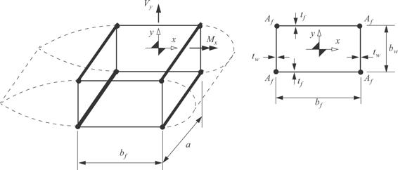— Fig. 11.33 Wing box beam of example 11.5.

Solution. The centroid and the shear center of the cross section coincide with the center of the box beam due to symmetry. The normal stress due to bending in the upper skin is calculated from the flexure formula; i.e.,

$\begin{align} σ_{z} = \frac{M_{x} (b_{w} / 2)}{I_{x x}}, & (a) \end{align}$ $math-2758.png$

where the second area moment of the cross section about the x-axis is

$\begin{align} I_{x x} = b_{w}^{2} A_{f} + \frac{1}{2} b_{f} b_{w}^{2} t_{f} + \frac{1}{6} b_{w}^{3} t_{w} = 1, 461.85 in .^{4} & (b) \end{align}$ $math-2759.png$

Hence, the bending normal stress in the upper skin is

$\begin{align} σ_{z} = - 18, 408.2 lb . / {in.}^{2} . & (c) \end{align}$ $math-2760.png$

The shear stress in the upper skin is determined from the analysis of the shear flow distribution around the contour of the cross section, which is shown in figure 11.34.

The shear flow in the upper skin is

$\begin{align} q_{3} = \frac{b_{w} t_{f} (b_{f} - 2 s_{3})}{4 I_{x x}} V_{y} 0 \leq s_{3} \leq b_{f} . & (d) \end{align}$ $math-2761.png$

The shear stress 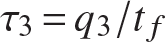$τ_{3} = q_{3} / t_{f}$ $math-2762.png$ , and its evaluation is

$\begin{align} τ_{3} = 55.5803 (24 - 2 s_{3}) lb . / {in.}^{2} 0 \leq s_{3} \leq 24 in . & (e) \end{align}$ $math-2763.png$

A rectangle with stringers in all four corners is shown with a positive shear cap V sub y aligned with the vertical y axis upward. The x axis is positive to the right. An equivalent representation of cap V sub y is shear flow through each of the sections, with the flow and path both beginning in the bottom left stringer and moving counterclockwise through the frame from s sub 1, q sub 1 to s sub 4, qu sub 4. A plot of the shear flow on the y axis and the path length on the x axis shows the shear starting at negative 650 pounds per inch at the first stringer, increasing linearly along the first branch to 650 pounds per inch at the second string 22 inches away. The second branch has a jump discontinuity from the first branch, beginning at 900 pounds per inch and arcing through a max of 1000 pounds per inch half-way through its length before returning to 900 pounds per inch at 38 inches. From here the third branch is the inverse of the first, moving from positive to negative, while the fourth branch is the inverse of the second, bottoming out at negative 1000, before returning to a final value of negative 900 at the end of path s at 72 inches. — Fig. 11.34 Shear flow distribution for the box beam of example 11.5.

Computing the maximum magnitude and the average value of this shear stress results in

$\begin{align} {|τ_{3}|}_{max} = 1, 333.93 lb / {in.}^{2} {(τ_{3})}_{ave} = \frac{1}{b_{f}} \int_{0}^{b_{f}} τ_{3} d s_{3} = 0 . & (f) \end{align}$ $math-2764.png$

The maximum magnitude of the shear stress in the upper skin is 7.25 percent of the magnitude of the bending normal stress. Moreover, the average value of the shear stress is zero in the upper skin. Hence, it is reasonable to neglect the effect of the shear stress on the buckling of the upper skin.

Assume the upper skin is a simply supported rectangular plate between the stringers and ribs. Actually, the stringer and ribs provide rotational constraint to the upper skin, but the assumption of no rotational constraint is conservative with respect to design. The critical compressive stress for simple support on all four edges of the upper skin underestimates its actual value. Equation (11.110) for the top cover skin is

$\begin{align} σ_{cr} = k_{c} π^{2} \frac{E}{12 (1 - v^{2})} {(\frac{t_{f}}{b_{f}})}^{2}, & (g) \end{align}$ $math-2765.png$

and eq. (11.114) for the compression buckling coefficient is

$\begin{align} k_{c} = {(\frac{m}{a / b_{f}} + \frac{a / b_{f}}{m})}^{2} m a positive integer to minimize k_{c} . & (a) \end{align}$ $math-2766.png$

The margin of safety is defined by

$\begin{align} M S = \frac{Excess strength}{Required strength} = \frac{σ_{cr} - |σ_{z}|}{|σ_{z}|} . & (11.119) \end{align}$ $math-2767.png$

The margin of safety (11.119) is positive for a feasible design, otherwise the design is infeasible. It should be a small positive value for a design of least weight. The computations for the margin of safety are listed in table 11.6.

A rib spacing of 16 in. is a feasible design with a slightly positive margin of safety.

■

Table 11.6 Margin of safety for selected rib spacings

a, in.	a/ $b_{f}$ $math-2768.png$	$k_{c}$ $math-2769.png$	$σ_{cr}$ $math-2770.png$ , lb./in. $^{2}$ $math-2771.png$	Margin of safety	Design
14	0.583	5.27905	20,708.6	0.12497	feasible
15	0.625	4.95063	19,420.2	0.05498	feasible
16	0.667	4.69444	18,415.3	0.000387	feasible
17	0.708	4.49482	17,632.20	−0.04215	infeasible
18	0.750	4.34028	17,026.0	−0.07509	infeasible
19	0.792	4.2223	16,563.2	−0.1002	infeasible

11.10 References

Brush, D. O., and B. O. Almroth. Buckling of Bars, Plates, and Shells. New York: McGraw-Hill, 1975, pp. 75–105.
Budiansky, B., and J. W. Hutchinson. “Dynamic Buckling of Imperfection-Sensitive Structures.” In Proceedings of the Eleventh International Congress of Applied Mechanics (Munich, Germany). 1964, pp. 639–643.
Budiansky, B. “Dynamic Buckling of Elastic Structures: Criteria and Estimates.” In Proceedings of an International Conference at Northwestern University (Evanston IL). New York and Oxford: Pergamon Press, 1966.
Gerard, G., and H. Becker. Handbook of Structural Stability: Part I, Buckling of Flat Plates. Technical Report NACA-TN 3781. Washington, DC: Office of Scientific and Technical Information, U.S. Department of Energy, 1957.
Koiter, W. T. “The Stability of Elastic Equilibrium.” PhD diss., Teehische Hoog School, Delft, The Netherlands, 1945. (English translation published as Technical Report AFFDL-TR-70-25, Air Force Flight Dynamics Laboratory, Wright-Patterson Air Force Base, OH, February 1970.)
National Advisory Committee for Aeronautics (NACA), Technical Note 3781 (NACA-TN-3781) July 1957. https://ntrs.nasa.gov/api/citations/1930084505/downloads/19930084505.pdf.
Ramberg, W., and Osgood, W. Description of Stress-Strain Curves by Three Parameters. Technical Report NACA-TN-902. Washington DC: NASA, 1943.
Southwell, Richard V. “On the Analysis of Experimental Observations in Problems of Elastic Stability.” Proc. Roy. Soc. London A, no. 135 (April 1932): 601–616.
Timoshenko, S. P., and J. M. Gere. Theory of Elastic Stability. New York: McGraw-Hill Book Company,1961, p.33.
Ugural A. C., and S. K. Fenster. Advanced Strength and Applied Elasticity, 4th ed.,Upper Saddle River, NJ: Pearson Education, Inc., Publishing as Prentice Hall Professional Technical Reference, 2003, pp. 472–490.

11.11 Practice exercises

1. An ideal column of length L is pinned at one end and fixed to a rigid bar of length a at the other end. The second end of the rigid bar is pinned on rollers. Refer to figure 11.35 Find the critical load P_cr and discuss the extreme cases of a→0 and a→∞.

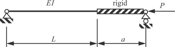
A two segment beam beam is shown pinned at each each. The first portion has stiffness cap E times cap I and is of length cap L, while the second portion of length cap a is completely rigid. A compressive load cap P is applied at the right-pinned end. — Fig. 11.35 Exercise 1.

2. The column shown in figure 11.36 is pinned at the left end and supported by an extensional spring of stiffness α at the loaded right end.

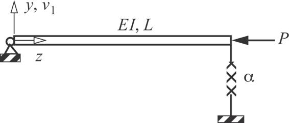
A beam is pinned at its left end and restricted from motion by a vertical spring of stiffness alpha at its tip. The z axis is aligned with the beam, while y is normal upwards, along with the displacement v sub 1. The beam has a stiffness of cap E times cap I and length cap L. — Fig. 11.36 Exercise 2.

a) Use the adjacent equilibrium method to show that the characteristic equation is

$\begin{array}{l} - k^{2} sin k L [- k^{2} + \frac{α L}{E I}] = 0 . \end{array}$ $math-2772.png$

b) Plot the critical load P_cr as a function of α, 0≤α. For what values of α will the column buckle in the Euler mode? (i.e., case A in figure 11.6).

A 6 bar truss forms a rectangular structure of width 1080 millimeters and height 810 millimeters. The the left two nodes, 3 on the bottom and 4 on the top, are both pinned, while the right two nodes, 1 on the bottom and 2 on the top, are free. A vertical force cap F is applied upward at node 2. — Fig. 11.37 Truss for exercise 3.

3. The statically indeterminate truss shown in figure 11.37 consists of six bars, labeled 1-2, 1-3, 1-4, 2-3, 2-4, and 3-4. It is subject to a vertical force F at joint number 2. The cross-sectional area of each bar is 2,000 mm², the second area moment of each bar is 160,000 mm⁴, and the modulus of elasticity of each bar is 75,000 N/mm².

a) Take bar force 1-4 as the redundant (i.e., $N_{1 - 4} = Q$ $math-2773.png$ ). Using Castigliano’s second theorem to determine the redundant Q in terms of the external load F.

b) Determine the value of F in kN to initiate buckling of the truss.

c) If the yield strength of the material is 400 MPa in tension, determine the value of F in kN to initiate yielding of the truss.

4. Bars 1-2, 2-3, and 2-4 of the truss shown figure 11.38 are unstressed at the ambient temperature. Only bar 1-2 is heated above the ambient temperature. Determine the increase in temperature, denoted by ΔT, of bar 1-2 to cause buckling of the truss. The cross section of each bar is a thin-walled tube with radius R = 13mm and wall thickness $t = 1.5 mm$ $math-2774.png$ . Take length L = 762mm. All three bars are made of the same material with properties $E = 75, 000 N / {mm}^{2}$ $math-2775.png$ and $α = 23 \times 1 0^{- 6} /^{°} C$ $math-2776.png$ .

A three bar truss is connected to pins at the end of each bar, and a shared central pin in the center. Node 1 is at the base of the first bar, which is vertical and connects it to node 2 a distance cap L away. Nodes 3 and 4 are both a distance cap L above node 2, and are the pinned points for the remaining two bars, with each forming a 30 degree angle with the horizontal on the right and left sides of the central node 2, respectively. The same truss structure is used, but now with the pin at the first node removed and replaced by reaction cap Q and resulting displacement q. The cross section of the bars is shown as a hollow circular tube of radius cap R and thickness t. Area is given as 2 pi times cap R times cap t. Area moment of inertia is given as pi times cap R cubed times t. 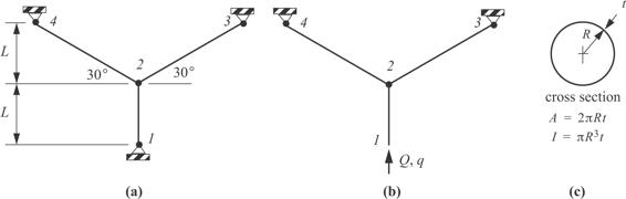— Fig. 11.38 Exercise 4. (a) three-bar truss, (b) base structure. (c) cross section of the bars.

5. Consider the wing spar in example 11.5. A counterclockwise torque $T = 6 \times 1 0^{6} lb.$ $math-2777.png$ -in. is specified to act at the root cross section in addition to the specified transverse shear force and bending moment. Determine the rib spacing, denoted by a, such that the margin of safety with respect to buckling of the upper skin is slightly positive. Report the value of a to two significant figures and the associated margin of safety. The margin of safety is defined by the formula

$\begin{array}{l} MS = \frac{1 - f_{b}}{f_{b}} where f_{b} = {(\frac{τ}{τ_{cr}})}^{2} + \frac{σ}{σ_{cr}} . \end{array}$ $math-2778.png$

Use the average value of the shear stress over the width of the upper skin for the shear stress τ in the margin of safety formula. Remember that dimension b is smaller than dimension a in the formula for the critical value of the shear stress, and that b is the width of the plate/skin on which the compressive normal stress acts in the formula for σ_cr.

1. Richard V. Southwell (1888–1970), British mathematician specializing in applied mechanics. In his article “On the Analysis of Experimental Observations in Problems of Elastic Stability”, he discussed the coordinates used in the plot to correlate the experimental data on elastic column buckling with linear theory.

Search

Text Color

Text Size

Margin Size

Font Type