11.2: Summary

Last updated
Save as PDF

Page ID: 95321

$ \newcommand{\vecs}[1]{\overset { \scriptstyle \rightharpoonup} {\mathbf{#1}} } $

$ \newcommand{\vecd}[1]{\overset{-\!-\!\rightharpoonup}{\vphantom{a}\smash {#1}}} $

$ \newcommand{\id}{\mathrm{id}}$ $ \newcommand{\Span}{\mathrm{span}}$

( \newcommand{\kernel}{\mathrm{null}\,}\) $ \newcommand{\range}{\mathrm{range}\,}$

$ \newcommand{\RealPart}{\mathrm{Re}}$ $ \newcommand{\ImaginaryPart}{\mathrm{Im}}$

$ \newcommand{\Argument}{\mathrm{Arg}}$ $ \newcommand{\norm}[1]{\| #1 \|}$

$ \newcommand{\inner}[2]{\langle #1, #2 \rangle}$

$ \newcommand{\Span}{\mathrm{span}}$

$ \newcommand{\id}{\mathrm{id}}$

$ \newcommand{\Span}{\mathrm{span}}$

$ \newcommand{\kernel}{\mathrm{null}\,}$

$ \newcommand{\range}{\mathrm{range}\,}$

$ \newcommand{\RealPart}{\mathrm{Re}}$

$ \newcommand{\ImaginaryPart}{\mathrm{Im}}$

$ \newcommand{\Argument}{\mathrm{Arg}}$

$ \newcommand{\norm}[1]{\| #1 \|}$

$ \newcommand{\inner}[2]{\langle #1, #2 \rangle}$

$ \newcommand{\Span}{\mathrm{span}}$ $ \newcommand{\AA}{\unicode[.8,0]{x212B}}$

$ \newcommand{\vectorA}[1]{\vec{#1}} % arrow$

$ \newcommand{\vectorAt}[1]{\vec{\text{#1}}} % arrow$

$ \newcommand{\vectorB}[1]{\overset { \scriptstyle \rightharpoonup} {\mathbf{#1}} } $

$ \newcommand{\vectorC}[1]{\textbf{#1}} $

$ \newcommand{\vectorD}[1]{\overrightarrow{#1}} $

$ \newcommand{\vectorDt}[1]{\overrightarrow{\text{#1}}} $

$ \newcommand{\vectE}[1]{\overset{-\!-\!\rightharpoonup}{\vphantom{a}\smash{\mathbf {#1}}}} $

$ \newcommand{\vecs}[1]{\overset { \scriptstyle \rightharpoonup} {\mathbf{#1}} } $

$ \newcommand{\vecd}[1]{\overset{-\!-\!\rightharpoonup}{\vphantom{a}\smash {#1}}} $

11.2.7 Summary

From this initial post-buckling analysis the results for the expansions of the load, displacements, and rotation are

$\begin{align} \frac{P}{P_{cr}} = 1 + \frac{ξ^{2}}{8} w (z) = - P_{cr} E A z + ξ^{2} w 2 (z) v (z) = ξ v_{1} (z) + ξ^{3} v 3 (z) ϕ (z) = ξ ϕ_{1} (z) + ξ^{3} ϕ 3 (z) . & (11.75) \end{align}$ $math-2575.png$

The strain of the centroidal axis is

$\begin{align} ε_{z z} = - \frac{P_{cr}}{E A} + ξ^{2} [\frac{d w_{2}}{d z} + \frac{1}{2} {(\frac{d v_{1}}{d z})}^{2}] . & (11.76) \end{align}$ $math-2576.png$

Rotation functions ϕ₁(z) and ϕ₃(z) are given by eqs. (11.38) and (11.69), respectively. Lateral displacement functions v₁(z) and v₃(z) are given by eqs. (11.39) and (11.70), respectively, and the axial displacement function w₂(z) is given by eq. (11.74).

Example 11.2 Numerical results for the initial post-buckling of the pinned-pinned column

Consider the column with a solid, rectangular cross section of height h and width b, where h < b. The radius of gyration is $r = \sqrt{I / A} = h / \sqrt{12}$ $math-2577.png$ . The strain at the bifurcation point is obtained from eq. (11.76) for ξ→0 is $- P_{cr} / (E A)$ $math-2578.png$ , and take this strain equal to $- 0.0006$ $math-2579.png$ . Since $P_{cr} = (π^{2} E I) / L$ $math-2580.png$ , we have

$\begin{align} \frac{P_{cr}}{E A} = \frac{π^{2} E I}{L^{2}} (\frac{1}{E A}) = \frac{π^{2}}{12} {(\frac{h}{L})}^{2} = 0.0006 . & (a) \end{align}$ $math-2581.png$

Hence, the span-to-thickness ratio $L / h = 37$ $math-2582.png$ .

The restriction on the magnitude of the expansion parameter ξ in the initial post-buckling analysis is based on the strain at the elastic limit of 7075-T6 aluminum alloy, which is about 0.0068. Let ${\bar{ε}}_{z z}$ $math-2583.png$ denote the strain of a line element parallel to the centroidal axis. It is the sum of the strain of centroidal axis ε_zz plus the strain due to bending. That is,

$\begin{align} {\bar{ε}}_{z z} = ε_{z z} + y (\frac{d ϕ}{d z}), & (b) \end{align}$ $math-2584.png$

where $(- h) / 2 \leq y \leq h / 2$ $math-2585.png$ and dϕ∕dz is the curvature of the centroidal axis. The magnitude of the maximum compressive strain in post-buckling occurs at midspan, $z = L / 2$ $math-2586.png$ , and $y = - h / 2$ $math-2587.png$ . That is,

$\begin{align} {\bar{ε}}_{z z} = ε_{z z} - {\frac{h}{2} (\frac{d ϕ}{d z})|}_{z = L / 2} . & (c) \end{align}$ $math-2588.png$

The expansion for the curvature at midspan is determined from eqs. (11.75), (11.38) and (11.69). The result is

$\begin{align} {\frac{d ϕ}{d z}|}_{z = L / 2} = [\frac{π}{L} sin (\frac{π z}{L})] ξ - {[\frac{π}{64 L} sin (\frac{3 π z}{L})] ξ^{3}|}_{z = L / 2} = \frac{π}{L} ξ + \frac{π}{64 L} ξ^{3} . & (d) \end{align}$ $math-2589.png$

Substitute $h = 0.270 L$ $math-2590.png$ and $P_{cr} = 0.0006 EA$ $math-2591.png$ in the expansions for the strains. The numerical evaluations of the strain in eq. (11.76) and the strain from bending are

$\begin{align} ε_{z z} = - 0.0006 - 0.000075 ξ^{2} - \frac{h}{2} (\frac{d ϕ}{d z}) = - 0.0424264 ξ - 0.000662193 ξ^{3} . & (e) \end{align}$ $math-2592.png$

The axial strain on the concave side of the bar at midspan is set equal to the elastic limit strain of $- 0.0068$ $math-2593.png$ . Thus,

$\begin{array}{l} {\bar{ε}}_{z z} = - 0.0006 - 0.042464 ξ - 0.000075 ξ^{2} - 0.000662913 ξ^{3} = - 0.0068 . \end{array}$ $math-2594.png$

The real root of the previous polynomial is the maximum value of parameter ξ, which is

$\begin{align} ξ_{max} = 0.14605 . & (f) \end{align}$ $math-2595.png$

For post-buckling coefficients a = 0 and $b = 1 / 8$ $math-2596.png$ , we get $P / P_{cr} = 1.0027$ $math-2597.png$ at $ξ = ξ_{max}$ $math-2598.png$ from eq. (11.54). There is a very small increase in the load during post-buckling. The lateral displacement of the column is determined from eqs. (11.75), (11.39), and (11.70), and it is a maximum at midspan. Evaluation of the maximum displacement is

$\begin{align} v_{max} = v (L / 2) = \frac{L ξ}{π} - \frac{7 L ξ^{2}}{64 π}, & (g) \end{align}$ $math-2599.png$

and $v_{max} = 0.04638 L$ $math-2600.png$ at $ξ = ξ_{max}$ $math-2601.png$ .

The axial displacement of the column is determined from eqs. (11.75) and (11.74). The shortening of distance between supports is

$\begin{align} Δ = - w (L) = L (0.0006) + (\frac{L}{4} + \frac{L (0.0006)}{8}) ξ^{2} . & (h) \end{align}$ $math-2602.png$

The shortening at buckling is $Δ_{cr} = {Δ|}_{ξ = 0} = L (0.0006)$ $math-2603.png$ , and the normalized shortening is defined by

$\begin{align} Δ / Δ_{cr} = 1 + 416.792 ξ^{2} . & (i) \end{align}$ $math-2604.png$

At $ξ = ξ_{max}$ $math-2605.png$ , $Δ / Δ_{cr} = 9.89$ $math-2606.png$ on the post-buckling path. The configuration of the column at ξ_max is shown in figure 11.8.

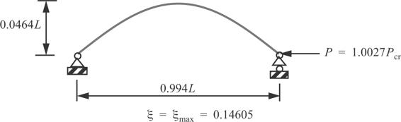
A buckled pinned-pinned beam shortens to a horizontal length of 0.994 times cap L, with a maximum vertical displacement at the center of 0.0464 times cap L. This occurs for a buckling load equal to 1.0027 times cap P sub cr, with the corresponding xi equal to xi sub max of 0.14605. — Fig. 11.8 Post-buckling configuration of the pinned-pinned column at the elastic limit strain.

The pre-buckling equilibrium path is determined from eq. (11.14) where $Δ = - w_{0} (L) = (P L) / (E A)$ $math-2607.png$ , or $P = (E A / L) Δ$ $math-2608.png$ . Divide by the critical load to get $P / P_{cr} = (E A / P_{cr}) (Δ / L)$ $math-2609.png$ . From eq. (a) the factor 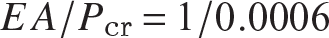$E A / P_{cr} = 1 / 0.0006$ $math-2610.png$ . Thus, $P / P_{cr} = Δ / (0.0006 L) = Δ / Δ_{cr}$ $math-2611.png$ on the pre-buckling equilibrium path.

With v sub max over cap L on the horizontal axis and cap P over cap P sub cr on the vertical axis, the vertical axis up to a value of 1, and a nearly linear path to either side of 1 are shown to be stable, while anything along the vertical axis above a value of 1 is shown as unstable. With delta over delta sub cr on the horizontal axis and cap P over cap P sub cr on the vertical axis, a line from the origin through the pint 1 1 is denoted as stable until the 1 1 point. Afterwards, stable states travel along a horizontal line for cap P over cap P sub cr equal to 1, while any points along the original line above 1 are now denoted as unstable. 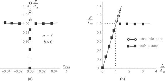— Fig. 11.9 Equilibrium paths for the pinned-pinned column subject to axial compression (a) on the load-deflection plot, and (b) on the load-shortening plot.

The load-deflection response is shown in figure 11.9(a), and the load-shortening response is shown in figure 11.9(b). The post-buckling behavior of the column is stable symmetric bifurcation, which is the same behavior as model A in article 10.1 on page 265. The load does not decrease in post-buckling. However, the increase in load is very small in post-buckling. From a practical point of view, the column is considered neutral in post-buckling.The structural stiffness is defined as dP∕dΔ. For post-buckling the structural stiffness is computed as

$\begin{array}{l} \frac{d P}{d Δ} = \frac{d P}{d ξ} \frac{d ξ}{d Δ} = (\frac{P_{cr}}{4} ξ) \frac{1}{2 (L / 4 + 0.0006 (L / 8)) ξ} = \frac{P_{cr}}{L (2 + 0.0006)} = \frac{E A (0.0006)}{L (2.0006)} = \frac{E A}{L} (0.0003) . \end{array}$ $math-2612.png$

The structural stiffness in pre-buckling is (EA)∕L. The ratio of the post-buckling stiffness to the pre-buckling stiffness is 0.0003, which indicates the dramatic loss of structural stiffness due to buckling.

■

From eq. (11.54) the perturbation expansion of the load in initial post-buckling is $P / P_{cr} = 1 + a ξ + b ξ^{2}$ $math-2613.png$ . The post-buckling coefficients a = 0 and b < 0 correspond to unstable symmetric bifurcation behavior illustrated by model B in article 10.2 on page 273. Post-buckling coefficient a ≠ 0 corresponds to asymmetric bifurcation behavior illustrated by model C in article 10.3 on page 277.

11.3 In-plane buckling of trusses

When a truss has all of its joints pinned, then there will be no interaction between the bending deflections of individual members. Hence the buckling load of the truss will be the load at which the weakest compression member buckles as an Euler column (case A in figure 11.6). However, when a truss is rigidly jointed, as in a frame, there will be interaction between bending deflections of neighboring members through rotation of the common joint. A rigid-jointed truss is stiffer than a pin-jointed truss, and therefore its buckling load is increased relative to the pin-jointed truss.

Example 11.3 Buckling of a two-bar truss

A symmetric truss consisting of two identical bars of length L are connected together by a hinge joint at the center of the truss. The opposite end of each bar connects to a separate hinge joint at a fixed support. Both supports are at a distance H below central joint. The central joint is subject to downward load Q whose corresponding displacement is denoted by q.

We consider a linear analysis and a nonlinear analysis for the stability of the truss, where Hooke’s law governs the material behavior in both analyses. The material of the bars is 7075-T6 aluminum alloy with a modulus of elasticity $E = 71, 000 N / {mm}^{2}$ $math-2614.png$ and yield strength of $σ_{yield} = 469 MPa$ $math-2615.png$ . The remaining numerical data are listed in table 11.2. From the data in table 11.2 the angle $β = 5.1 6^{°}$ $math-2616.png$ . A small value of β characterizes a shallow truss configuration.

The cross section of the example truss A two-bar truss is shown to be pinned on each end and in the center. The bars are angled above the horizontal by beta, with each element of length cap L and the center being cap H above the horizontal resulting in a sine beta equal to cap H over cap L. A downward force cap Q and resulting displacement q are applied at the central pin. Section A-A is a solid square of height h and width b. 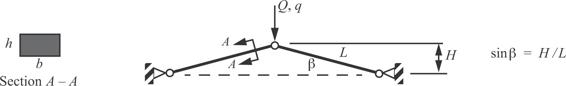— Fig. 11.10 A shallow truss horizontally constrained between fixed points.

Table 11.2 Numerical data for the truss in figure 11.10

Length of truss bars L, mm	300	Width of truss bar b, mm	25
Truss rise above supports H, mm	27	Area of truss bar A, mm²	450
Thickness of truss bar h, mm	18	Second area moment I, mm⁴	12,150

Axial strain-displacement relation. The strain-displacement relation (11.7) for each bar is

$\begin{align} ε_{z z} = \frac{d w}{d z} + \frac{1}{2} {(\frac{d v}{d z})}^{2}, & (a) \end{align}$ $math-2617.png$

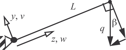
One of the trusses from the previous figure is shown with a local z axis and w displacement along the bar, as well as a normal y axis and v displacement upward normal to the bar. At the tip cap L away from the frame’s origin along the z-axis, a downward displacement q is shown, angled beta from the negative y direction. — Fig. 11.11 Left-hand bar of the truss.

where the axial displacement is denoted by w(z) and the lateral displacement is denoted by v(z). Consider the bar on the left-hand side of the truss as shown in figure 11.11. At the fixed end where z = 0, $w (0) = v (0) = 0$ $math-2618.png$ . At the end of the bar where z = L the axial displacement and the lateral displacement are related to the downward displacement q of the movable joint by $w (L) = - q sin β$ $math-2619.png$ and $v (L) = - q cos β$ $math-2620.png$ , respectively. The axial strain in a truss bar is uniform along its length, which means that the displacements are linear in coordinate z. Linear displacement functions for each displacement satisfying the end conditions are,

$\begin{align} w (z) = (- q sin β) (z / L) v (z) = (- q cos β) (z / L) . & (b) \end{align}$ $math-2621.png$

Substitute eq. (b) for the displacement functions into eq. (a) to get the strain-displacement relation

$\begin{align} ε_{z z} = (sin β) (\frac{- q}{L}) + \frac{1}{2} ({cos}^{2} β) {(\frac{q}{L})}^{2} . & (c) \end{align}$ $math-2622.png$

Substitute $sin β = H / L$ $math-2623.png$ , and $cos β = (\sqrt{L^{2} - H^{2}}) / L$ $math-2624.png$ into eq. (c) to get

$\begin{align} ε_{z z} = \frac{H}{L} (\frac{- q}{L}) + \frac{(L^{2} - H^{2})}{2 L^{2}} {(\frac{- q}{L})}^{2} . & (d) \end{align}$ $math-2625.png$

Numerical evaluation of eq. (d) is

$\begin{align} ε_{z z} = (- 3 \times 1 0^{- 4} / mm) q + (5.51056 \times 1 0^{6} / {mm}^{2}) q^{2} . & (e) \end{align}$ $math-2626.png$

The strain energy of the truss is

$\begin{align} U = 2 (\frac{1}{2} E A L ε_{z z}^{2}), & (f) \end{align}$ $math-2627.png$

in which the leading factor of 2 accounts for the two bars. Castigliano’s first theorem determines the force Q by

$\begin{align} Q = \frac{\partial U}{\partial q} = 2 E A L ε_{z z} \frac{\partial ε_{z z}}{\partial q} . & (g) \end{align}$ $math-2628.png$

Substitute eq. (d) for the strain into eq. (f) to get

$\begin{align} Q = 2 E A [\frac{H^{2}}{L^{3}} q - \frac{3 H (L^{2} - H^{2})}{2 L^{5}} q^{2} + \frac{{(L^{2} - H^{2})}^{2}}{2 L^{7}} q^{3}] . & (h) \end{align}$ $math-2629.png$

Numerical evaluation of eq. (h) is

$\begin{align} Q = (1, 725.3 N / mm) q - (95.0736 N / {mm}^{2}) q^{2} + (1.16424 N / {mm}^{3}) q^{3} . & (i) \end{align}$ $math-2630.png$

In-plane buckling of the truss bars based on linear analysis. The expressions for the axial strain (e) and applied load (h) reduce to

$\begin{align} ε_{z z} = \frac{H}{L} (\frac{- q}{L}) = (- 3 \times 1 0^{- 4} {mm}^{- 1}) q, and Q = 2 E A [\frac{H^{2}}{L^{3}} q] = (1, 725.3 N / mm) q . & (j) \end{align}$ $math-2631.png$

The axial force in each bar is given by

$\begin{align} N = E A ε_{z z} = (- 9, 585 N / mm) q . & (k) \end{align}$ $math-2632.png$

The Euler buckling force $P_{E} = (π^{2} E I) / L^{2} = 94.60 kN$ $math-2633.png$ . Set $- N = P_{E}$ $math-2634.png$ to find the displacement for in-plane buckling of the truss bars $q = 9.87 mm$ $math-2635.png$ . The corresponding load $Q = 17.028 kN$ $math-2636.png$ .

Equations (i) and (j) are plotted on the graph of load Q versus displacement q in figure 11.12. As the load is increased from zero on the nonlinear path (i) a limit point load of 9.038 kN at a displacement of 11.5 mm is encountered. As discussed in article 10.5 a dynamic snap-through motion occurs at the limit load that eventually (with damping) settles to a displacement of 58.65 mm. The linear response path (j) is the straight line in figure 11.12, and the load causing in-plane buckling of the truss bars is 17.028 kN. Thus, the critical load for this structure is at the limit point.

■

11.4 Geometrically imperfect column

Consider a uniform, pinned-pinned column that is slightly crooked under no load. The initial shape under no load is described by the function v₀(z). The column is subject to a centric, axial compressive load P. The lateral displacement of the column is denoted by v(z), so that v(z) = v₀(z) when P = 0. Moment equilibrium of the free body diagram for a segment of the column shown in figure 11.13 is

$\begin{align} M_{x} - v P = 0 . & (11.77) \end{align}$ $math-2637.png$

A plot with q in millimeters on the horizontal axis and cap Q in kilo Newtons on the vertical axis shows the two-bar truss response. An initial linear portion can stretch from the origin to a point at 9.7 millimeters and 17.028 kilo Newtons, but the standard path will follow a sinusoidal path through its first peak at 11.5 millimeters and 9.038 kilo Newtons. It can then continue to follow the sinusoidal path, with is symmetric about the q axis, or it could perform a dynamic snap through, which jumps from this first peak to the same cap Q value on the next upward portion of the curve at 48.56 millimeters and 9.038 kilo Newtons. 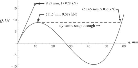— Fig. 11.12 Load-displacement responses of the two-bar truss from linear and nonlinear analyses.

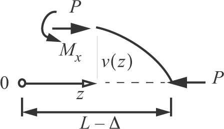
Looking at the right edge of a column now length cap L minus delta, the compressive load cap P is opposed by an equal compressive load cap P internally, as well as a counterclockwise moment cap M sub x, resulting from the upward displacement v of z at the point in question. — Fig. 11.13 FBD of the right-hand part of a pinned-pinned column.

The bending moment in the column is zero under no load, so we write the material law for bending as

$\begin{align} M_{x} = E I (\frac{d ϕ}{d z} - \frac{d ϕ_{0}}{d z}), & (11.78) \end{align}$ $math-2638.png$

where ϕ₀(z) is the rotation of the initial shape of the column. For small slopes of the slightly deflected column the rotations are related to the lateral displacements by

$\begin{align} ϕ (z) = - (\frac{d v}{d z}) ϕ_{0} (z) = - (\frac{d v_{0}}{d z}) . & (11.79) \end{align}$ $math-2639.png$

Hence, the bending moment becomes

$\begin{align} M_{x} = - E I (\frac{d^{2} v}{d z^{2}} - \frac{d^{2} v_{0}}{d z^{2}}) . & (11.80) \end{align}$ $math-2640.png$

Substitute the bending moment from eq. (11.80) into the moment equilibrium equation (11.77) to get

$\begin{align} - E I (\frac{d^{2} v}{d z^{2}} - \frac{d^{2} v_{0}}{d z^{2}}) - v P = 0 . & (11.81) \end{align}$ $math-2641.png$

Equation (11.81) is arranged to the form

$\begin{align} \frac{d^{2} v}{d z^{2}} + k^{2} v = \frac{d^{2} v_{0}}{d z^{2}}, & (11.82) \end{align}$ $math-2642.png$

where $k^{2} = P / (E I)$ $math-2643.png$ . Take the initial shape of the column 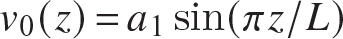$v_{0} (z) = a_{1} sin (π z / L)$ $math-2644.png$ , where a₁ is the amplitude of the initial shape at midspan. Then the differential equation for v(z) is

$\begin{align} \frac{d^{2} v}{d z^{2}} + k^{2} v = - a_{1} {(\frac{π}{L})}^{2} sin (π z / L) 0 < z < L . & (11.83) \end{align}$ $math-2645.png$

The boundary conditions are 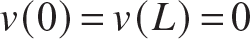$v (0) = v (L) = 0$ $math-2646.png$ . The solution of the differential equation (11.83) subject to boundary conditions is

$\begin{align} v (z) = \frac{a_{1}}{1 - {(\frac{k L}{π})}^{2}} sin (\frac{π z}{L}) 0 \leq z \leq L . & (11.84) \end{align}$ $math-2647.png$

The term $k^{2} L^{2} / π^{2} = P / P_{cr}$ $math-2648.png$ where the critical load of the perfect structure is $P_{cr} = (π^{2} E I) / L^{2}$ $math-2649.png$ . It is convenient to measure the deflection of the imperfect column under load with respect to its original unloaded state. That is, let δ define the additional displacement at midspan by 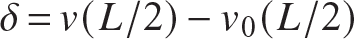$δ = v (L / 2) - v_{0} (L / 2)$ $math-2650.png$ . Hence,

$\begin{align} δ = a_{1} \frac{(\frac{P}{P_{cr}})}{1 - (\frac{P}{P_{cr}})} . & (11.85) \end{align}$ $math-2651.png$

The load-displacement response is sketched in figure 11.14. Note that $| δ | \to \infty$ $math-2652.png$ as P→P_cr for a₁ ≠ 0. That is, for a non-zero value of the imperfection amplitude, the displacement gets very large as the axial force approaches the buckling load of the perfect column. Also, the imperfect column deflects in the direction of imperfection (e.g., if a₁ > 0, then δ > 0).

With deflection lowercase delta on the horizontal axis and cap P over cap P sub cr on the vertical axis, a horizontal dotted line passes through a value of 1, corresponding to P sub cr equal to pi squared time cap E times cap I all over cap L squared. The deflection curve initially hugs the vertical axis and dotted lines asymptotically, but will gradually move down and to the right as imperfection a sub 1 is increased. 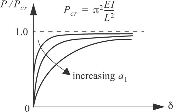— Fig. 11.14 Load-deflection response plots for geometrically imperfect columns.

An arbitrary initial shape is represented by a Fourier Sine series as

$\begin{align} v_{0} (z) = a_{1} sin \frac{π z}{L} + a_{2} sin \frac{2 π z}{L} + \dots . & (11.86) \end{align}$ $math-2653.png$

Timoshenko and Gere (1961) show the solution for $δ (z) = v (z) - v_{0} (z)$ $math-2654.png$ is

$\begin{align} δ (z) = \frac{P}{P_{cr}} [\frac{a_{1}}{1 - P / P_{cr}} sin (\frac{π z}{L}) + \frac{a_{2}}{2^{2} - P / P_{cr}} sin (\frac{2 π z}{L}) + \dots] . & (11.87) \end{align}$ $math-2655.png$

For P < P_cr as P→P_cr, the first term dominates the solution for δ(z). Thus, for P near $P_{cr}$ $math-2656.png$

$\begin{align} δ_{c} = δ (\frac{L}{2}) \sim \frac{P / P_{cr}}{1 - P / P_{cr}} a_{1} . & (11.88) \end{align}$ $math-2657.png$

The buckling behavior of a long, straight column subject to centric axial compression (the perfect column) is classified as stable symmetric bifurcation. As such it is imperfection insensitive. Refer to the discussions in article 10.1.5 on page 272 and article 10.2.1 on page 275. Even for a well manufactured column whose geometric imperfections are small, and with the load eccentricity small, the displacements become excessive as the axial compressive force P approaches the critical load $P_{cr}$ $math-2658.png$ of the perfect column. Hence, the critical load determined from the analysis of the perfect column is meaningful in practice.

11.4.1 Southwell plot

Rearrange eq. (11.88) as follows: $δ_{c} (1 - P / P_{cr}) = (P / P_{cr}) a_{1}$ $math-2659.png$ , then $δ_{c} - (P / P_{cr}) δ_{c} = (P / P_{cr}) a_{1}$ $math-2660.png$ . Divide the last by P to get

$\begin{align} \frac{δ_{c}}{P} = \frac{(δ_{c} + a_{1})}{P_{cr}} . & (11.89) \end{align}$ $math-2661.png$

We plot δ_c∕P versus δ_c from eq. (11.89) in figure 11.15, which is called the Southwell plot (Southwell, 1932).¹ The Southwell plot is very useful for determining $P_{cr}$ $math-2662.png$ from test data in the elastic range. As $P \to P_{cr}$ $math-2663.png$ , $P < P_{cr}$ $math-2664.png$ , δ becomes large and the data ( 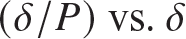$(δ / P) vs. δ$ $math-2665.png$ ) tends to plot on a straight line. Extrapolating this straight line back to toward the ordinate axis (δ∕P) one can estimate a₁ and $P_{cr}$ $math-2666.png$ . It is more difficult to determine $P_{cr}$ $math-2667.png$ by the load-deflection curve obtained in experiments as illustrated in figure 11.16.

Deflection lower case delta sub c on the horizontal axis and lower case delta sub c over cap P on the vertical axis are used within the plot. A line of slope 1 over cap P sub cr is shown passing through an x-intercept of negative a sub 1, and a vertical intercept of a sub 1 over cap P sub cr. The experimental data drops asymptotically along the vertical axis above the line, but approaches is asymptotically as lower case delta increases. 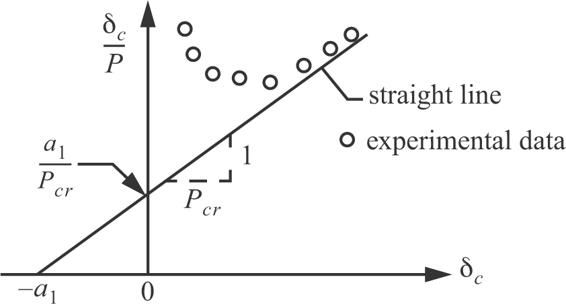— Fig. 11.15 Southwell plot.

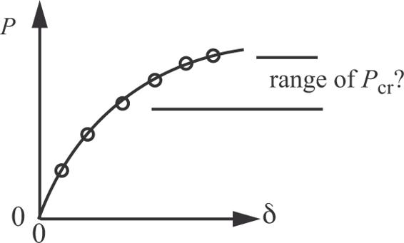
The theory and experimental data track well together, with slight variations apparent as points can be seen to be just above or just below the line in certain places. — Fig. 11.16 Load-deflection plot from test data.

11.5 Column design curve

Consider the pinned-pinned uniform column whose critical load is given by $P_{cr} = π^{2} (E I / L^{2})$ $math-2668.png$ . Let A denote the cross-sectional area of the column. At the onset of buckling the critical stress is defined as

$\begin{align} σ_{cr} = P_{cr} / A = (π^{2} E I) / (A L^{2}) . & (11.90) \end{align}$ $math-2669.png$

The second area moment is I = r²A, where r denotes the minimum radius of gyration of the cross section. For the rectangular section shown in figure 11.17, 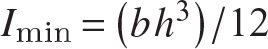$I_{min} = (b h^{3}) / 12$ $math-2670.png$ and A = bh, so that 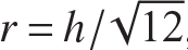$r = h / \sqrt{12}$ $math-2671.png$ , where $0 < h < b$ $math-2672.png$ . Thus, the critical stress becomes

$\begin{align} σ_{cr} = π^{2} \frac{E}{{(L / r)}^{2}} . & (11.91) \end{align}$ $math-2673.png$

and L∕r is called the slenderness ratio. The slenderness ratio is the column length divided by a cross-sectional dimension significant to bending.

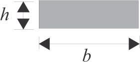
A rectangle of height h and width b. — Fig. 11.17

For any set of boundary conditions define the effective length KL by the formula

$\begin{align} P_{cr} = π^{2} \frac{E I}{{(K L)}^{2}} . & (11.92) \end{align}$ $math-2674.png$

The effective lengths for the four standard boundary conditions are as follows:

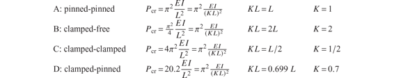
$\begin{array}{l} \begin{matrix} A: pinned-pinned & P_{cr} = π^{2} \frac{E I}{L^{2}} = π^{2} \frac{E I}{{(K L)}^{2}} & K L = L & K = 1 \\ B: clamped-free & P_{cr} = \frac{π^{2}}{4} \frac{E I}{L^{2}} = π^{2} \frac{E I}{{(K L)}^{2}} & K L = 2 L & K = 2 \\ C: clamped-clamped & P_{cr} = 4 π^{2} \frac{E I}{L^{2}} = π^{2} \frac{E I}{{(K L)}^{2}} & K L = L / 2 & K = 1 / 2 \\ D: clamped-pinned & P_{cr} = 20.2 \frac{E I}{L^{2}} = π^{2} \frac{E I}{{(K L)}^{2}} & K L = 0.699 L & K = 0.7 \end{matrix} \end{array}$ $math-2675.png$

The definition of effective length uses case A boundary conditions as a reference. The concept of effective length accounts for boundary conditions other than simple support, or pinned-pinned end conditions.

The column curve is a plot of the critical stress versus the effective slenderness ratio (i.e., $σ_{c r} versus K L / r$ $math-2676.png$ ). For elastic column buckling under all boundary conditions

$\begin{align} σ_{cr} = \frac{π^{2} E}{{(\frac{K L}{r})}^{2}}, & (11.93) \end{align}$ $math-2677.png$

which is a hyperbola that depends only on the modulus of elasticity E of the material. This equation governing elastic buckling is called the Euler curve, and columns that buckle in the elastic range are called long columns. See figure 11.18.

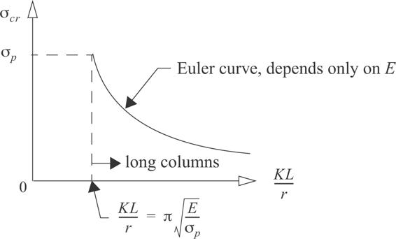
A plot shows cap K times cap L over r on the horizontal axis, with sigma sub cr on the vertical axis. The Euler curve begins at a point where cap K times cap L over r is equal to pi times the square root of cap E over sigma sub p, and sigma sub p on the vertical axis. The curve then moves downward with a gradually increasing slope until it begins to approach the horizontal axis asymptotically. — Fig. 11.18 Column curve for elastic buckling.

11.5.1 Inelastic buckling

The column curve equation, eq. (11.93), is valid up to the proportional limit of the material, denoted by σ_p. The proportional limit is defined as the stress where the compressive stress-strain curve of the material deviates from a straight line. If the stress at the onset of buckling is greater than the proportional limit, then the column is said to be of intermediate length, and the Euler formula, eq. (11.93), cannot be used. The proportional limit is difficult to measure from test data because its definition is based on the deviation from linearity. In particular, the compressive stress-strain curves for aluminum alloys typically used in aircraft construction do not exhibit a very pronounced linear range. For aluminum alloys a material law developed by Ramberg and Osgood (1943) is often used to describe the nonlinear compressive stress-strain curve. The Ramberg-Osgood equation is a three-parameter fit to the compressive stress-strain curves of aluminum alloys. From the experimental compressive stress-strain curve the slope near the origin is the modulus of elasticity E. The stress where the secant line drawn from the origin with slope 0.85 E intersects the stress-strain curve is denoted σ_0.85.The stress where a second secant line drawn from the origin with slope 0.7 E intersects the stress-strain curve is denoted by σ_0.7. These data are depicted in figure 11.19. Note that the compressive normal strain corresponding to the stress σ_0.7 is usually about the 0.2 percent offset yield strain for the material. Hence, stress σ_0.7 is close to the 0.2 percent offset yield stress of the aluminum alloy. The Ramberg-Osgood equation is

A stress strain curve is shown with strain on the horizontal axis and stress on the vertical axis. An initial linear portion is shown with slope cap E, but then gradually begins to level off as the strain is increased. As the slope levels off, the line connecting each point to the origin decreases in slope through 0.85 times cap E and eventually showing a value of 0.7 times cap E at a strain of 0.002. The stress at each of these points is denoted by sigma with a subscript equal to the coefficient of cap E. — Fig. 11.19 Data used to fit the compression stress-strain curve of aluminum alloys.

$\begin{align} ε = \frac{σ}{E} [1 + \frac{3}{7} {(\frac{σ}{σ_{0.7}})}^{n - 1}], & (11.94) \end{align}$ $math-2678.png$

where the shape parameter n is given by

$\begin{align} n = 1 + ln (\frac{17}{7}) / ln (\frac{σ_{0.7}}{σ_{0.85}}) . & (11.95) \end{align}$ $math-2679.png$

Equation (11.94) is re-written as

$\begin{align} \frac{E ε}{σ_{0.7}} = \frac{σ}{σ_{0.7}} + \frac{3}{7} {(\frac{σ}{σ_{0.7}})}^{n}, & (11.96) \end{align}$ $math-2680.png$

and is plotted as $σ / σ_{0.7}$ $math-2681.png$ versus $(E ε) / σ_{0.7}$ $math-2682.png$ for various values of the shape parameter n, This plot is shown in figure 11.20. Some approximate values for common aluminum alloys are listed in table 11.3.

Table 11.3 Ramberg-Osgood parameters for selected aluminum alloys

AL	E in 10 $^{6}$ $math-2683.png$ psi	$σ_{0.7}$ $math-2684.png$ in 10 $^{3}$ $math-2685.png$ psi	n
2014-T6	10.6	60	20
2024-T4	10.6	48	10
6061-T6	10.0	40	30
7075-T6	10.4	73	20

The horizontal axis represents cap E time epsilon, all over sigma sub 0.7, and sigma over sigma sub 0.7 on the vertical axis. Lines for n values of 2, 5, 10, 20, and 50 are shown. N equal 2 is approximately linear, while each increase in n results in the line curving downward, and the resulting corner moving up and to the left. By n equal 50, the curve is occurring around 0.9 on the horizontal axis, and asymptotically approaching a horizontal line through 1 on the vertical axis. The ends of each line continue to drop as n is increased, with n equal to 20 and 50 being approximately 1 by the end. All lines, however, pass through a point a 1.4 on the horizontal axis and 0.95 on the vertical axis. 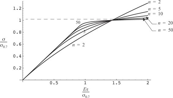— Fig. 11.20 A normalized plot of the Ramberg-Osgood material law for various values of the shape parameter n.

From the Ramberg-Osgood equation, eq. (11.94), the local slope of the compressive stress-strain curve is determined as a function of the stress. This slope of the compressive stress-strain curve is called the tangent modulus (i.e., $\frac{d σ}{d ε} = E_{t}$ $math-2686.png$ where E_t is the tangent modulus). Differentiate eq. (11.94) to get

$\begin{align} d ε = \frac{d σ}{E} + \frac{3}{7} \frac{n σ^{n - 1}}{E σ_{0.7}^{n} - 1} d σ \frac{d ε}{d σ} = \frac{1}{E_{t}} = \frac{1}{E} + \frac{3}{7} \frac{n}{E} {(\frac{σ}{σ_{0.7}})}^{n - 1} . & (11.97) \end{align}$ $math-2687.png$

Thus, the tangent modulus is

$\begin{align} E_{t} = \frac{E}{1 + \frac{3}{7} n {(\frac{σ}{σ_{0.7}})}^{n - 1}} . & (11.98) \end{align}$ $math-2688.png$

For intermediate length columns it has been demonstrated by extensive testing that the critical stress is reasonably well predicted using the Euler curve, eq. (11.93), with the modulus of elasticity replaced by the tangent modulus. This inelastic buckling analysis is called the tangent modulus theory. That is,

$\begin{align} σ_{cr} = π^{2} \frac{E_{t}}{{(\frac{K L}{r})}^{2}} . & (11.99) \end{align}$ $math-2689.png$

Now substitute eq. (11.98) for the tangent modulus in the latter equation, noting that $σ = σ_{cr}$ $math-2690.png$ , to get

$\begin{align} σ_{cr} = \frac{π^{2}}{{(\frac{K L}{r})}^{2}} [\frac{E}{1 + \frac{3}{7} n {(\frac{σ_{cr}}{σ_{0.7}})}^{n - 1}}] . & (11.100) \end{align}$ $math-2691.png$

After division by σ_0.7, eq. (11.100) can be written as

$\begin{align} \frac{σ_{cr}}{σ_{0.7}} + \frac{3}{7} n {(\frac{σ_{cr}}{σ_{0.7}})}^{n} = \frac{1}{{[\frac{(K L / r)}{π \sqrt{E / σ_{0.7}}}]}^{2}} . & (11.101) \end{align}$ $math-2692.png$

A plot of the column curve given by eq. (11.101) is shown in figure 11.21.

The horizontal axis represents cap K times cap L over r, all over the expression pi times square root of cap E over sigma sub 0.7. The vertical axis shows sigma sub cr over sigma sub 0.7. Lines for n equal to 2, 5, 10, 20, and 50 are shown, with a set of dotted lines corresponding to n equal infinity. For n equal infinity, the line would be equal to one for values between zero and 1 on the horizontal axis, and then follow a downward curve that asymptotically approaches the horizontal axis by a value of 3.5. For larger values of n, the curve resembles the n equal infinity curve by coming down the vertical axis rapidly, having a very low slope between 0 and 1 on the vertical axis, then following the asymptotic curve after 1. However, as n is decreased, the line gradually moves away from the vertical axis and loses its inboard levelling, instead taking shallower asymptotic curves and joining the n equals infinity curve at later and later points. 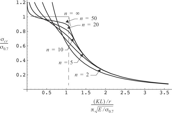— Fig. 11.21 Column curves for a Ramberg-Osgood material law with different shape factors.

11.6 Bending of thin plates

Recall that bars and beams are structural elements characterized by having two orthogonal dimensions, say the thickness and width, that are small compared to the third orthogonal dimension, the length. Thin plates, both flat and curved, are common structural elements in flight vehicle structures, and they are characterized by one dimension being small, say the thickness, with respect to the other two orthogonal dimensions, say the width and length. A thin, rectangular, flat plate shown in figure 11.22 is referenced to Cartesian axes x, y, and z, where the x-direction is parallel to the length, the y-direction is parallel to the width, and the z-axis is parallel to the thickness of the plate. We denote the length of the plate by a, the width by b, and the thickness by t, and $0 \leq x \leq a$ $math-2693.png$ , $0 \leq y \leq b$ $math-2694.png$ , and $- t / 2 \leq z \leq t / 2$ $math-2695.png$ . The plane with z = 0 is the midsurface, or reference surface, of the plate.

A infinitesimal stress element is shown with primary stresses from plate theory. These stresses include only the in-plane normal stresses and shear stresses, denoted by x and y subscripts. A full infinitesimal stress element is shown, with a normal stress sigma and two shear stresses tau on each face, with the sigma subscript of x, y, or z denoting its face, and tau’s subscripts denoting its face and direction, in that order. Finally, the infinitesimal stress element is shown within a larger place of width b, length a, and thickness t. The plate has a coordinate frame in its top right corner, with x along the length, y along the width, and z through the thickness. Both a and b are shown to be much greater than t. 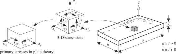— Fig. 11.22 Illustration of the nomenclature and primary stresses for a flat, rectangular plate.

A beam resists the transverse loads, or lateral loads, primarily by the longitudinal normal stress σ_x, and the so-called lateral stresses σ_y, σ_z, τ_yx, and τ_yz are assumed to be negligible. Transverse loads, acting in the z-direction applied to the plate are primarily resisted by the in-plane stress components σ_x, σ_y, and τ_xy. Transverse shear stresses τ_xz and τ_yz are necessary for force equilibrium in the z-direction under transverse loads, but are smaller in magnitude with respect to the in-plane stresses. In plate theory, the transverse normal stress σ_z is very small with respect to the in-plane normal stresses and, hence, is neglected. Bending of thin plates is discussed in many texts on plate theory; for example, see Ugural and Fenster (2003). Only some elements of the plate bending theory are discussed here. The assumptions of the linear theory for thin plates are as follows:

1. The deflection of the midsurface is small with respect to the thickness of the plate, and the slope of the deflected midsurface is much less than unity.

2. Straight lines normal to the midsurface in the undeformed plate remain straight and normal to the midsurface in the deformed plate, and do not change length.

3. The normal stress component σ_z is negligible with respect to the in-plane normal stresses and is neglected in Hooke’s law.

Now consider the deformation, or strains, caused by the normal stresses. Hooke’s law for the normal stresses and strains in a three-dimensional state of stress is

$\begin{align} \begin{aligned} ε_{x} & = \frac{1}{E} (σ_{x} - v σ_{y} - v σ_{z}) \\ ε_{y} & = \frac{1}{E} (- v σ_{x} + σ_{y} - v σ_{z}) \\ ε_{z} & = \frac{1}{E} (- v σ_{x} - v σ_{y} + σ_{z}) \end{aligned}, & (11.102) \end{align}$ $math-2696.png$

where E is the modulus of elasticity and v is Poisson’s ratio. From assumption 3 the thickness normal stress $σ_{z}$ $math-2697.png$ is assumed negligible and is set to zero in Hooke’s law. From assumption 2 the thickness normal strain ε_z = 0, because the line element normal to the midsurface does not change length. Since the normal stress σ_z is also assumed to vanish, the third of eq. (11.102) leads to a contradiction. Hence, the third equation of Hooke’s law is neglected. The material law for the in-plane normal strains and stresses for thin plates is

$\begin{align} \begin{aligned} ε_{x} & = \frac{1}{E} (σ_{x} - v σ_{y}) \\ ε_{y} & = \frac{1}{E} (- v σ_{x} + σ_{y}) \end{aligned} . & (11.103) \end{align}$ $math-2698.png$

Consider two cases of pure bending of a plate or a beam subject to moment M. In the first case the cross section is compact with dimension b nearly equal to thickness t, and in the second case dimension b is much larger than thickness t. In the first case the structure is a beam, and in the second case it is a plate. In pure bending the neutral axis of the beam deforms into an arc of a circle with radius ρ, and the normal strain in the x-direction is $ε_{x} = z / ρ$ $math-2699.png$ . Note that we assumed that the x-axis coincided with the neutral axis in the undeformed beam. Hence, longitudinal line elements above the neutral axis, z > 0, are stretched, and line elements below the neutral axis, z < 0, are compressed. In the case of a beam, the normal stress in the y-direction, σ_y, is also very small and is neglected with respect to the longitudinal normal stress σ_x. That is, the beam resists the applied bending moment by the longitudinal normal stress σ_x. Since σ_y = 0, we get from Hooke’s law, eq. (11.103), that

$\begin{align} \begin{gathered} σ_{x} = E ε_{x} \\ ε_{y} = - v ε_{x} = - \frac{v}{ρ} z = - \frac{z}{(\frac{ρ}{v})} \end{gathered} . & (11.104) \end{align}$ $math-2700.png$

Hence, the longitudinal normal stress is the modulus of elasticity times the longitudinal normal strain, and the normal strain in the y-direction is just Poisson’s ratio times the longitudinal normal strain. The form of the last expression for ε_y in eq. (11.104) shows that the line elements in the cross section parallel to the y-axis before deformation also bend into circular arcs. The line element parallel to the y-direction at z = 0 in the undeformed beam has a radius of curvature of $\frac{ρ}{v}$ $math-2701.png$ in the deformed beam. This transverse curvature is called anticlastic curvature, and is illustrated in figure 11.23.

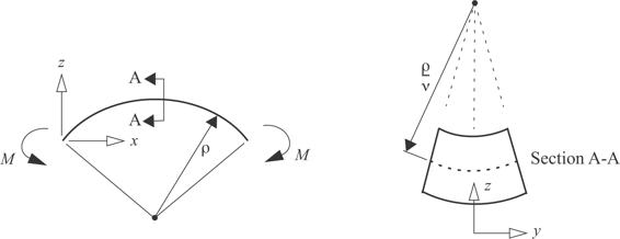
And arc is shown at a radius rho from the center of curvature, and counteracting moments on each end. A slice cap A dash cap A is denoted at the center, while a local coordinate system at the left end has an x axis towards the right and z upward. Cross-section cap A dash cap A is shown as a segment of the arc, at a radius rho over nu. — Fig. 11.23 Pure bending of a beam in the x- z plane and the associated anticlastic curvature of its cross section.

Now consider pure bending of a plate under the same moment M, where now the dimension b is much larger than thickness t. In this case experiments show that the transverse line elements remain straight over the central section of the plate, so that the anticlastic curvature is suppressed. In this central section of the plate the transverse normal stress ε_y is non-zero. However, the transverse normal stress must vanish at the free edges at y = 0 and y = b, so that anticlastic curvature develops only in narrow zones near the free edges to adjust to vanishing of the normal stress σ_y at the free edges. In the central portion of the plate, the associated normal strain is zero. The suppression of anticlastic curvature is characterized by the vanishing of the normal strain ε_y. Hence from Hooke’s law, eq. (11.103), for ε_y = 0 we get

$\begin{align} σ_{x} = \frac{E}{1 - v^{2}} ε_{x} σ_{y} = v σ_{x} . & (11.105) \end{align}$ $math-2702.png$

Since the denominator in the expression for σ_x is positive but less than unity, the plate is stiffer than the beam owing to the presence of the non-zero transverse normal stress σ_y to help in resisting the applied moment. Compare eqs. (11.104) and (11.105) for the normal stress σ_x. The quantity $E / (1 - v^{2})$ $math-2703.png$ is an effective modulus of the plate.

Search

Text Color

Text Size

Margin Size

Font Type