10.4: Creating Subplots

Sometimes we want to show multiple plots in one figure window without placing them on top of each other. For that, we use subplot. A subplot divides one figure window into a grid of smaller plotting areas. The general format is:

 

subplot(r, c, n)

The first input, r, is the number of rows of plots. The second input, c, is the number of columns of plots. The third input, n, tells MATLAB which subplot position should be active. MATLAB counts the positions across each row, starting from the upper-left corner. For example, for a 2-by-2 subplot:

subplot command	Layout created	Active position
subplot(2,2,1)	2 rows by 2 columns	upper-left plot
subplot(2,2,2)	2 rows by 2 columns	upper-right plot
subplot(2,2,3)	2 rows by 2 columns	lower-left plot
subplot(2,2,4)	2 rows by 2 columns	lower-right plot

Subplots are helpful when you want to compare related graphs side by side. For example, you might use subplots to compare experimental results from different test cases, temperatures from different cities, or the same function plotted with different numbers of points.

Example \(\PageIndex{1}\)

Comparing 10 Points and 20 Points

The following example uses subplots to compare what happens when we plot sin(x) using 10 points versus 20 points.

% Demonstrating subplots using a for loop
clear; clc; clf;


for i = 1:2
    x = linspace(0, 2*pi, 10*i);
    y = sin(x);
    
    
    subplot(1, 2, i)
    plot(x, y, 'ko')
    ylabel('sin(x)')
    xlabel('x')
    title(sprintf('%d Points', 10*i))
end

 

Solution

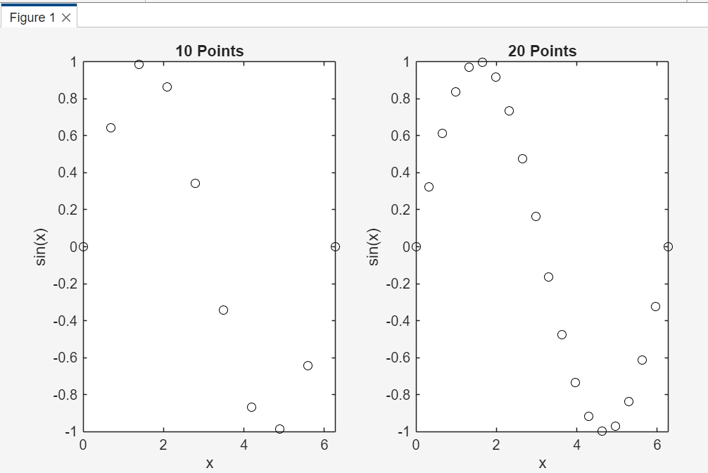
The first subplot uses 10 points and the second subplot uses 20 points. With more points, the shape of the sine wave becomes easier to recognize. This is an important lesson: plots depend on the data points used to create them.

 

Keeping the Same Axis Limits

When we compare two or more subplots, we often want the axes to use the same scale. If each subplot has a different x-axis or y-axis range, the comparison can become misleading. A curve may look steeper, flatter, larger, or smaller simply because MATLAB chose different axis limits.

For this reason, when subplots are meant to be compared directly, it is a good habit to use the same x-limits and y-limits for all of them. The functions xlim and ylim control the visible limits of the x-axis and y-axis.

 

xlim([xmin xmax])

ylim([ymin ymax])

You can also use axis to set both x and y limits at the same time.

 

axis([xmin xmax ymin ymax])

For example, the following script compares sin(x) and cos(x) in two subplots while keeping the same axis limits.

Example \(\PageIndex{2}\)

Comparing sin(x) and cos(x) in two subplots while keeping the same axis limits.

% Subplots with matching axis limits
clear; clc; clf;


x = linspace(0, 2*pi, 50);
y1 = sin(x);
y2 = cos(x);


subplot(1, 2, 1)
plot(x, y1, 'b')
title('sin(x)')
xlabel('x')
ylabel('y')
xlim([0 2*pi])

ylim([-1.5 1.5])
grid on


subplot(1, 2, 2)
plot(x, y2, 'r')
title('cos(x)')
xlabel('x')
ylabel('y')
xlim([0 2*pi])

ylim([-1.5 1.5])
grid on

 

Solution

 

 

 

Note

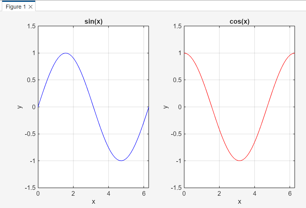
Good comparison habit: When subplots are used for comparison, keep the same axis limits unless there is a specific reason not to. This helps the reader compare shapes and values fairly.

Another useful command is sgtitle, which adds one title above all subplots in a figure.

 

sgtitle('Comparison of Sine and Cosine')

Use individual titles for each subplot when each graph needs its own label, and use sgtitle when the entire figure needs one shared title.