
Determine Initial and Final Values
- Page ID
- 101113
\( \newcommand{\vecs}[1]{\overset { \scriptstyle \rightharpoonup} {\mathbf{#1}} } \)
\( \newcommand{\vecd}[1]{\overset{-\!-\!\rightharpoonup}{\vphantom{a}\smash {#1}}} \)
\( \newcommand{\dsum}{\displaystyle\sum\limits} \)
\( \newcommand{\dint}{\displaystyle\int\limits} \)
\( \newcommand{\dlim}{\displaystyle\lim\limits} \)
\( \newcommand{\id}{\mathrm{id}}\) \( \newcommand{\Span}{\mathrm{span}}\)
( \newcommand{\kernel}{\mathrm{null}\,}\) \( \newcommand{\range}{\mathrm{range}\,}\)
\( \newcommand{\RealPart}{\mathrm{Re}}\) \( \newcommand{\ImaginaryPart}{\mathrm{Im}}\)
\( \newcommand{\Argument}{\mathrm{Arg}}\) \( \newcommand{\norm}[1]{\| #1 \|}\)
\( \newcommand{\inner}[2]{\langle #1, #2 \rangle}\)
\( \newcommand{\Span}{\mathrm{span}}\)
\( \newcommand{\id}{\mathrm{id}}\)
\( \newcommand{\Span}{\mathrm{span}}\)
\( \newcommand{\kernel}{\mathrm{null}\,}\)
\( \newcommand{\range}{\mathrm{range}\,}\)
\( \newcommand{\RealPart}{\mathrm{Re}}\)
\( \newcommand{\ImaginaryPart}{\mathrm{Im}}\)
\( \newcommand{\Argument}{\mathrm{Arg}}\)
\( \newcommand{\norm}[1]{\| #1 \|}\)
\( \newcommand{\inner}[2]{\langle #1, #2 \rangle}\)
\( \newcommand{\Span}{\mathrm{span}}\) \( \newcommand{\AA}{\unicode[.8,0]{x212B}}\)
\( \newcommand{\vectorA}[1]{\vec{#1}} % arrow\)
\( \newcommand{\vectorAt}[1]{\vec{\text{#1}}} % arrow\)
\( \newcommand{\vectorB}[1]{\overset { \scriptstyle \rightharpoonup} {\mathbf{#1}} } \)
\( \newcommand{\vectorC}[1]{\textbf{#1}} \)
\( \newcommand{\vectorD}[1]{\overrightarrow{#1}} \)
\( \newcommand{\vectorDt}[1]{\overrightarrow{\text{#1}}} \)
\( \newcommand{\vectE}[1]{\overset{-\!-\!\rightharpoonup}{\vphantom{a}\smash{\mathbf {#1}}}} \)
\( \newcommand{\vecs}[1]{\overset { \scriptstyle \rightharpoonup} {\mathbf{#1}} } \)
\(\newcommand{\longvect}{\overrightarrow}\)
\( \newcommand{\vecd}[1]{\overset{-\!-\!\rightharpoonup}{\vphantom{a}\smash {#1}}} \)
\(\newcommand{\avec}{\mathbf a}\) \(\newcommand{\bvec}{\mathbf b}\) \(\newcommand{\cvec}{\mathbf c}\) \(\newcommand{\dvec}{\mathbf d}\) \(\newcommand{\dtil}{\widetilde{\mathbf d}}\) \(\newcommand{\evec}{\mathbf e}\) \(\newcommand{\fvec}{\mathbf f}\) \(\newcommand{\nvec}{\mathbf n}\) \(\newcommand{\pvec}{\mathbf p}\) \(\newcommand{\qvec}{\mathbf q}\) \(\newcommand{\svec}{\mathbf s}\) \(\newcommand{\tvec}{\mathbf t}\) \(\newcommand{\uvec}{\mathbf u}\) \(\newcommand{\vvec}{\mathbf v}\) \(\newcommand{\wvec}{\mathbf w}\) \(\newcommand{\xvec}{\mathbf x}\) \(\newcommand{\yvec}{\mathbf y}\) \(\newcommand{\zvec}{\mathbf z}\) \(\newcommand{\rvec}{\mathbf r}\) \(\newcommand{\mvec}{\mathbf m}\) \(\newcommand{\zerovec}{\mathbf 0}\) \(\newcommand{\onevec}{\mathbf 1}\) \(\newcommand{\real}{\mathbb R}\) \(\newcommand{\twovec}[2]{\left[\begin{array}{r}#1 \\ #2 \end{array}\right]}\) \(\newcommand{\ctwovec}[2]{\left[\begin{array}{c}#1 \\ #2 \end{array}\right]}\) \(\newcommand{\threevec}[3]{\left[\begin{array}{r}#1 \\ #2 \\ #3 \end{array}\right]}\) \(\newcommand{\cthreevec}[3]{\left[\begin{array}{c}#1 \\ #2 \\ #3 \end{array}\right]}\) \(\newcommand{\fourvec}[4]{\left[\begin{array}{r}#1 \\ #2 \\ #3 \\ #4 \end{array}\right]}\) \(\newcommand{\cfourvec}[4]{\left[\begin{array}{c}#1 \\ #2 \\ #3 \\ #4 \end{array}\right]}\) \(\newcommand{\fivevec}[5]{\left[\begin{array}{r}#1 \\ #2 \\ #3 \\ #4 \\ #5 \\ \end{array}\right]}\) \(\newcommand{\cfivevec}[5]{\left[\begin{array}{c}#1 \\ #2 \\ #3 \\ #4 \\ #5 \\ \end{array}\right]}\) \(\newcommand{\mattwo}[4]{\left[\begin{array}{rr}#1 \amp #2 \\ #3 \amp #4 \\ \end{array}\right]}\) \(\newcommand{\laspan}[1]{\text{Span}\{#1\}}\) \(\newcommand{\bcal}{\cal B}\) \(\newcommand{\ccal}{\cal C}\) \(\newcommand{\scal}{\cal S}\) \(\newcommand{\wcal}{\cal W}\) \(\newcommand{\ecal}{\cal E}\) \(\newcommand{\coords}[2]{\left\{#1\right\}_{#2}}\) \(\newcommand{\gray}[1]{\color{gray}{#1}}\) \(\newcommand{\lgray}[1]{\color{lightgray}{#1}}\) \(\newcommand{\rank}{\operatorname{rank}}\) \(\newcommand{\row}{\text{Row}}\) \(\newcommand{\col}{\text{Col}}\) \(\renewcommand{\row}{\text{Row}}\) \(\newcommand{\nul}{\text{Nul}}\) \(\newcommand{\var}{\text{Var}}\) \(\newcommand{\corr}{\text{corr}}\) \(\newcommand{\len}[1]{\left|#1\right|}\) \(\newcommand{\bbar}{\overline{\bvec}}\) \(\newcommand{\bhat}{\widehat{\bvec}}\) \(\newcommand{\bperp}{\bvec^\perp}\) \(\newcommand{\xhat}{\widehat{\xvec}}\) \(\newcommand{\vhat}{\widehat{\vvec}}\) \(\newcommand{\uhat}{\widehat{\uvec}}\) \(\newcommand{\what}{\widehat{\wvec}}\) \(\newcommand{\Sighat}{\widehat{\Sigma}}\) \(\newcommand{\lt}{<}\) \(\newcommand{\gt}{>}\) \(\newcommand{\amp}{&}\) \(\definecolor{fillinmathshade}{gray}{0.9}\)When solving second-order differential equation problems, it's crucial to determine two initial conditions. In the context of circuit problems, these initial conditions represent the voltage across a component and its derivative at a specific point in time, usually at t = 0.
For instance, consider an RLC circuit. The voltage across a capacitor (C) and the current through an inductor (L) depend on the initial conditions of the circuit. When analyzing such circuits, v(0) represents the voltage across the capacitor at the initial time t=0, while v′(0) represents the derivative of voltage with respect to time at t=0. Similarly, for an inductor, i(0) represents the current through the inductor at t=0, and i′(0) represents the derivative of current with respect to time at t=0.
v(0) signifies the initial charge stored in the capacitor, while v′(0) indicates the rate of change of voltage across the capacitor at t=0, reflecting the initial energy stored in the inductor. For the inductor, i(0) represents the initial current flowing through it, while i′(0) reflects the rate of change of current at t=0, indicating the initial energy stored in the inductor's magnetic field. These initial conditions are essential for solving the differential equations governing the circuit's behavior and determining both transient and steady-state responses.
In circuits containing capacitors and inductors, the voltage across capacitors and the current through inductors are continuous. This principle ensures that the voltage across the capacitor right before the switch (at t=0−) and immediately after the switch (at t=0+) remains the same.
This continuity arises from the physical properties of these components. Capacitors resist sudden changes in voltage, maintaining a consistent voltage level. Similarly, inductors resist abrupt changes in current, ensuring that the current flowing through them remains constant. As a result, when a switch is toggled in a circuit containing capacitors and inductors, the voltage across the capacitor exhibits continuity, ensuring smooth transitions and stability in the circuit's behavior.
vc(0-) = vc(0+) and iL(0-) = iL(0+)
This fundamental principle is crucial for analyzing and designing circuits, as it helps ensure proper operation and prevents voltage or current spikes that could potentially damage circuit components.
To determine the change in capacitor voltage and inductor current, it's often necessary to utilize the fundamental relationships between voltage (V) and current (I) for capacitors and inductors, along with Kirchhoff's Current Law (KCL) and Kirchhoff's Voltage Law (KVL). An example can help illustrate these concepts.
After being closed for an extended duration, the capacitor behaves as an open circuit, while the inductor acts as a short wire. At t=0, the switch is opened. The task is to determine the initial values before and after t=0, the rates of their changes immediately after t=0, and their eventual final values.

Solution
Initially, we analyze the circuit t<0 when the switch is closed for a long time. During this period, the inductor behaves like a wire, while the capacitor is open, as depicted below. We use source transformation to convert the current source to a voltage source. Our objective is to determine the current flowing through the inductor wire iL(0-) and the voltage across the capacitor Vc(0-).
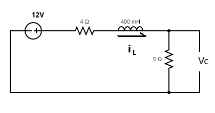
The initial current flowing through the inductor is determined by the current within the loop iL(0−), which equals 12/(4Ω+5Ω) = 1.33A. Similarly, the initial voltage across the capacitor can be found using a voltage divider, yielding Vc(0−) = 6.67V, equivalent to the voltage across the 5Ω resistor.
As time approaches infinity, the inductor effectively transforms into a short wire, while the capacitor reverts to an open circuit. Consequently, the circuit becomes open, resulting in a final current of iL = 0A. Additionally, the voltage of Vc settles at 12V across the entire circuit, as there is no voltage difference in an open circuit configuration.

Next, we address how to determine the initial rate of change of current and voltage, denoted as iL′(0+) andVC′(0+) respectively. This can be accomplished by applying Kirchhoff's Voltage Law (KVL) to the circuit for t>0.
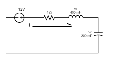
The V-i relation for the capacitor is iC(0+) = C⋅VC′(0+). Since the current in a series circuit remains constant iC(0+)/C = iL(0+)/C = 1.33A, we have
VC′(0+) = iC(0+)/C = iL(0+)/C = 1.33/0.2 = 6.66 V/S
Following the clockwise current direction, the KVL equation is given by
−12+iL(0+)×4+VL(0+)+VC(0+)=0.
Notably, Vc(0+) = Vc(0−) = 6.67V and iL(0+) = 1.33A, we can find the initial voltage of the inductor VL(0+)
VL(0+) = 0 V
Utilizing the fundamental math model of the inductor, we can solve the rate of change inductor current iL′(0+).
iL′(0+) = VL(0+)/L = 0