8.4: Parallel Circuit Analysis

Kirchhoff's current law (KCL) is the operative rule for parallel circuits. It states that the sum of all currents entering and exiting a node must equal zero. Alternately, it can be stated as the sum of currents entering a node must equal the sum of currents exiting that node. As a pseudo formula:

$$\sum I \rightarrow = \sum I \leftarrow \label{3.6}$$

A similar situation occurs in AC parallel circuits to that seen AC series circuits; namely that it appears that KCL (like KVL) is “broken”. That is, a simplistic summing of the magnitudes of the currents might not balance. Once again, this is because the summation must be a vector summation, paying attention to the phase angles of each separate current.

It is possible to drive a parallel circuit with multiple current sources. These sources will add in much the same way that voltage sources in series add, that is, polarity and phase must be considered. Ordinarily, voltage sources with differing values are not placed in parallel as this violates the basic rule of parallel circuits (voltage being the same across all components).

The current divider rule remains valid for AC parallel circuits. Given two components, $Z_1$ and $Z_2$, and a current feeding them, $I_T$, the current through one of the components will equal the total current times the ratio of the opposite component over the sum of the impedance of the pair.

$$i_1 = i_T \frac{Z_2}{Z_1 + Z_2} \label{3.7}$$

This rule is convenient in that the parallel equivalent impedance need not be computed, but remember, it is valid only when there are just two components involved.

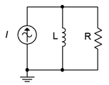
When analyzing a parallel circuit, if it is being driven by a voltage source, then this same voltage must appear across each of the individual components. Ohm's law can then be used to determine the individual currents. According to KCL, the total current exiting the source must be equal to the sum of these individual currents. For example, in the circuit shown in Figure $\PageIndex{1}$, the voltage $E$ must appear across both $R$ and $L$. Therefore, the currents must be $i_L = E / X_L$ and $i_R = E / R$, and $i_{total} = i_L + i_R$. $i_{total}$ can also be found be determining the parallel equivalent impedance of $R$ and $X_L$, and then dividing this into $E$. This technique can also be used in reverse in order to determine a resistance or reactance value that will produce a given total current: dividing the source by the current yields the equivalent parallel impedance. As one of the two is already known, the known component can be used to determine the value of the unknown component via Equation 3.3.3.

Example $\PageIndex{1}$

Determine the currents in the circuit shown in Figure $\PageIndex{1}$ if the source is $10\angle 0^{\circ}$ volts peak, $X_L = j2 k\Omega$ and $R = 1 k\Omega$

Figure $\PageIndex{1}$: A simple parallel RL circuit.

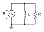
The same voltage must appear across all elements in a parallel connection. In this case that's $10\angle 0^{\circ}$ volts peak. The two branch currents are found via Ohm's law:

$$i_L = \frac{v}{Z} \nonumber$$

$$i_L = \frac{10\angle 0^{\circ} V}{j2 k\Omega} \nonumber$$

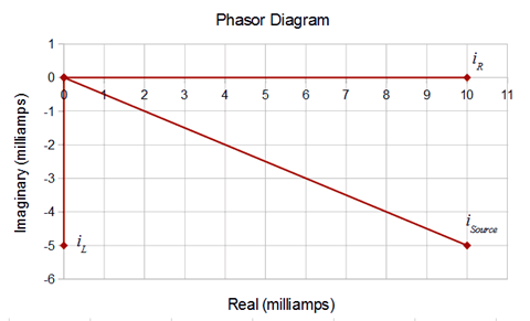
$$i_L = 5E-3\angle −90^{\circ} A \nonumber$$

$$i_R = \frac{v}{Z} \nonumber$$

$$i_R = \frac{10\angle 0^{\circ} V}{1k \Omega} \nonumber$$

$$i_R = 10E-3\angle 0^{\circ} A \nonumber$$

The source current is the sum of the these two currents, or $11.18E−3\angle −26.6^{\circ}$ amps. This can be verified by determining the equivalent parallel impedance and then applying Ohm's law:

$$Z_T = \frac{Z_1\times Z_2}{Z_1+Z_2} \nonumber$$

$$Z_T = \frac{1k \Omega\times j 2k \Omega}{1k \Omega+j 2k \Omega} \nonumber$$

$$Z_T = 894\angle 26.6^{\circ} \Omega \nonumber$$

As a side note, in rectangular form this is $800 + j400$, meaning that this parallel combination is equivalent to a series combination of an 800 ohm resistance and a 400 ohm inductive reactance. Continuing with Ohm's law, we have:

$$i_{Source} = \frac{v}{Z_T} \nonumber$$

$$i_{Source} = \frac{10\angle 0^{\circ} V}{894\angle 26.6^{\circ} \Omega} \nonumber$$

$$i_{Source} = 11.18E-3\angle −26.6^{\circ} A \nonumber$$

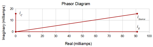
A phasor diagram of the currents is shown in Figure $\PageIndex{2}$, below.

Figure $\PageIndex{2}$: Phasor diagram of currents in the circuit of Figure $\PageIndex{1}$.

Current Measurement in the Laboratory

At this point, a practical question arises; how do we verify these currents in the laboratory? After all, the preeminent measurement tool is the oscilloscope, and these are designed to measure voltage, not current. While it is possible to obtain current measurement probes, a simple method to measure current is to use a small current sensing resistor with a standard oscilloscope setup. We have seen already that the voltage across a resistor must be in phase with the current through it. Therefore,

whatever phase angle we see on a resistor's voltage, its current phase angle must be the same. The idea is to simply insert a resistor into the branch of which we wish to measure the current. As long as the resistance is much smaller than the impedance seen in the rest of that branch, it will have little impact on the precise value of the current. We can then place a probe across this sensing resistor to read its voltage. Ohm's law is then be used to determine the current's magnitude, while the phase angle is obtaining directly from the oscilloscope (again, because the sensing resistor's voltage must be in phase with its current, and thus the voltage phase angle is equal to the current phase angle). This technique will be illustrated in the simulation portion of the next example problem.

Example $\PageIndex{2}$

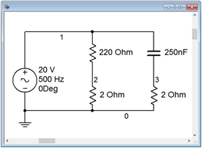
Determine the branch currents in the circuit of Figure $\PageIndex{3}$.

Figure $\PageIndex{3}$: Circuit for Example $\PageIndex{2}$.

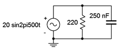
The first step is to determine the capacitive reactance.

$$X_C =− j \frac{1}{2 \pi f C} \nonumber$$

$$X_C =− j \frac{1}{2 \pi 500 Hz 250 nF} \nonumber$$

$$X_C \approx − j 1273\Omega \nonumber$$

Both the resistor and capacitor will see 20 volts peak from the source. Their currents can be determined via Ohm's law:

$$i_C = \frac{v}{X_C} \nonumber$$

$$i_C = \frac{20 V}{1273\angle −90^{\circ} \Omega} \nonumber$$

$$i_C \approx 15.71E-3\angle 90^{\circ} A \nonumber$$

$$i_R = \frac{v}{R} \nonumber$$

$$i_R = \frac{20 V}{220\angle 0^{\circ} \Omega} \nonumber$$

$$i_R \approx 90.91E-3\angle 0^{\circ} A \nonumber$$

The source current is the sum of these two currents, or $92.26E−3\angle 9.8^{\circ}$ amps. The source current may also be determined by dividing the source voltage by the equivalent parallel impedance, as follows.

$$Z_T = \frac{Z_1 \times Z_2}{Z_1+Z_2} \nonumber$$

$$Z_T = \frac{220 \Omega\times (− j 1273\Omega)}{220 \Omega − j 1273 k \Omega} \nonumber$$

$$Z_T = 216.8\angle −9.8^{\circ} \Omega \nonumber$$

$$i_{Source} = \frac{v}{Z_T} \nonumber$$

$$i_{Source} = \frac{20 \angle 0^{\circ} V}{216.8\angle −9.8^{\circ} \Omega} \nonumber$$

$$i_{Source} = 92.26E-3\angle 9.8^{\circ} A \nonumber$$

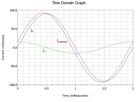
A time domain plot of the currents is illustrated in Figure $\PageIndex{4}$ along with a phasor plot in Figure $\PageIndex{5}$. Note that the source current is close in both amplitude and phase to the resistor current. By comparison, the capacitor current is considerably smaller and with an obvious leading phase shift.

Figure $\PageIndex{4}$: Current waveforms for the circuit of Figure $\PageIndex{3}$.

Figure $\PageIndex{5}$: Phasor diagram for the circuit of Figure $\PageIndex{3}$.

Computer Simulation

The circuit of Figure $\PageIndex{3}$ is captured in a simulator as shown in Figure $\PageIndex{6}$. Individual 2 ohm resistors are used to sense the currents in the resistor and capacitor branches. These sensing resistors are inserted directly above ground for convenience of measure. In this way a differential measurement is not needed.

Figure $\PageIndex{6}$: Circuit of Figure $\PageIndex{3}$ in a simulator with added current sensing resistors.

The value of a sensing resistor needs to be considerably smaller than the impedance of the branch in which it is inserted. Two orders of magnitude (i.e., less than 1 %) would be a good place to start. While even smaller values will increase accuracy, from a practical standpoint in the lab, such tiny resistor values would produce extremely small voltages that would be difficult to measure with great accuracy.

Figure $\PageIndex{7}$: Simulation results for the circuit of Figure $\PageIndex{6}$.

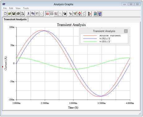
A basic transient analysis is then performed as shown in Figure $\PageIndex{7}$. The results of the simulation are in tight agreement with the plot of Figure $\PageIndex{4}$. Note that the plotted resistor and capacitor “currents” are, in fact, the voltages across the associated sensing resistors (nodes 2 and 3) divided by 2 (ohms), in direct application of Ohm's law. Not only does the simulation verify the results computed earlier, it also validates the concept of using small current sensing resistors in the laboratory.

Example $\PageIndex{3}$

Determine the the branch currents in the circuit of Figure $\PageIndex{8}$. Use the source voltage as the reference $(\angle 0^{\circ})$.

Figure $\PageIndex{8}$: Circuit for Example $\PageIndex{3}$.

Although this circuit is drawn a little differently than the prior examples, it remains a simple parallel circuit with just two nodes. Therefore, each element sees a 2 volt peak potential. Ohm's law will suffice to find the three component currents. These are then added to find the source current. Their reference directions are right-to-left given the source's polarity.

$$i_C = \frac{v}{X_C} \nonumber$$

$$i_C = \frac{2\angle 0^{\circ} V}{12 \angle −90^{\circ} \Omega} \nonumber$$

$$i_C \approx 0.1667\angle 90^{\circ} A \nonumber$$

$$i_L = \frac{v}{X_L} \nonumber$$

$$i_L = \frac{2\angle 0^{\circ} V}{8\angle 90 ^{\circ} \Omega} \nonumber$$

$$i_L = 0.25 \angle −90 ^{\circ} A \nonumber$$

$$i_R = \frac{v}{R} \nonumber$$

$$i_R = \frac{2\angle 0^{\circ} V}{10\angle 0^{\circ} \Omega} \nonumber$$

$$i_R = 0.2\angle 0^{\circ} A \nonumber$$

The sum of these three currents is approximately $0.2167\angle −22.6^{\circ}$ amps. This value can be verified by finding the combined parallel impedance. Using Equation 3.3.3 it can be shown that this impedance is $9.231\angle 22.6^{\circ} \Omega$. Thus,

$$i_{Source} = \frac{v}{Z} \nonumber$$

$$i_{Source} = \frac{2\angle 0^{\circ} V}{9.231\angle 22.6^{\circ} \Omega} \nonumber$$

$$i_{Source} \approx 0.2167\angle −22.6^{\circ} A \nonumber$$

A phasor diagram showing the vector summation of the currents is illustrated in Figure $\PageIndex{9}$.

Figure $\PageIndex{9}$: Current phasor diagram for the circuit of Figure $\PageIndex{8}$.

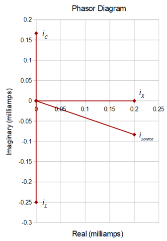
Note that $i_C$ and $i_L$ are in perfect opposition as expected. Subtracting the magnitude of $i_C$ from $i_L$ leaves us with the precise vertical component of the source current.

If a parallel circuit is driven by a current source, as shown in Figure $\PageIndex{10}$, there are two basic methods of solving for the component currents. The first method is to use the current divider rule. If desired, the component voltage can then be found using Ohm's law. An alternate method involves finding the parallel equivalent impedance first and then using Ohm's law to determine the voltage (remember, being a parallel circuit, there is only one common voltage). Given the voltage, Ohm's law can be used to find the current through one component. To find the current through the other, either Ohm's law can be applied a second time or KCL may be used; subtracting the current through the first component from the source current. If there are more than two components, usually the second method would be the most efficient course of action.

Figure $\PageIndex{10}$: Parallel network driven by a current source.

It is worth noting that both methods described above will yield the correct answers. One is not “more correct” than the other. We can consider each of these as a separate solution path; that is, a method of arriving at the desired end point. In general, the more complex the circuit, the more solution paths there will be. This is good because one path may be more obvious to you than another. It also allows you a means of crosschecking your work.

Example $\PageIndex{4}$

Determine the currents in the circuit of Figure $\PageIndex{10}$ if the source is 300 milliamps peak at 10 kHz, $R$ is $750 \Omega$ and $L$ is 15 mH.

The first step is to determine the inductive reactance.

$$X_L = j 2\pi f L \nonumber$$

$$X_L = j 2\pi 10 kHz15 mH \nonumber$$

$$X_L \approx j 942.4\Omega \nonumber$$

The current divider rule can be used to find the current through the resistor.

$$i_R = i_{Source} \frac{X_L}{R+X_L} \nonumber$$

$$i_R = 0.3\angle 0^{\circ} A \frac{942.4\angle 90 ^{\circ} \Omega}{750\angle 0^{\circ} \Omega +942.4\angle 90^{\circ} \Omega} \nonumber$$

$$i_R = 0.2347\angle 38.5 ^{\circ} A \nonumber$$

KVL can be used to find the remaining current through the inductor as the source current must equal the sum of the inductor and resistor currents. Therefore:

$$i_L = i_{Source} − i_R \nonumber$$

$$i_L = 0.3\angle 0^{\circ} A −0.2347\angle 38.5^{\circ} A \nonumber$$

$$i_L = 0.1868\angle −51.5^{\circ} A \nonumber$$

This value could also have been obtained by applying the current divider rule a second time:

$$i_L = i_{Source} \frac{R}{R+X_L} \nonumber$$

$$i_L = 0.3\angle 0^{\circ} A \frac{750\angle 0^{\circ} \Omega}{750\angle 0^{\circ} \Omega +942.4\angle 90 ^{\circ} \Omega} \nonumber$$

$$i_L = 0.1868\angle −51.5^{\circ} A \nonumber$$

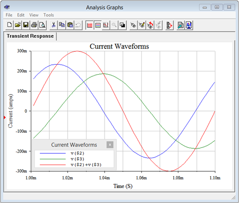
A time domain plot of the current waveforms is shown in Figure $\PageIndex{11}$.

Figure $\PageIndex{11}$: Current waveforms for the circuit of Example $\PageIndex{4}$.

From the plot it is apparent that the inductor and resistor currents do indeed add up to the source current. Further, the current through the inductor is lagging, as expected.

Computer Simulation

The circuit of Example $\PageIndex{4}$ is captured in a simulator as shown in Figure $\PageIndex{12}$. A pair of 1 ohm current sensing resistors have been added. By using 1 ohm, the sensing voltage will have the same magnitude as the current, with no scaling required.

Figure $\PageIndex{12}$: Circuit of Example $\PageIndex{4}$ in a simulator.

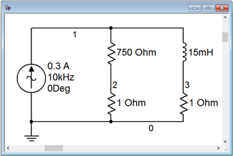
A transient analysis is performed, plotting the voltages at nodes 2 and 3 along with their sum (the source current). The results are shown in Figure $\PageIndex{3}$. The plot is delayed for a millisecond in order to avoid the initial power-up transient. The results are in full agreement with the plot of Figure $\PageIndex{11}$.

Figure $\PageIndex{13}$: Results of the transient response simulation for the circuit of Example $\PageIndex{5}$.

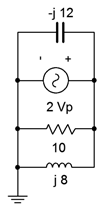
Example $\PageIndex{5}$

Determine the branch currents in the circuit of Figure $\PageIndex{14}$. Use the current source as the time reference (i.e., $\angle 0^{\circ}$).

Figure $\PageIndex{14}$: Circuit for Example $\PageIndex{5}$.

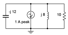
Instead of using repeated current dividers here, we can instead find the equivalent impedance and then apply Ohm's law to determine the system voltage. Each branch current may be obtained by dividing this voltage by the impedance of that branch; a quick application of Ohm's law.

The system impedance is computed through Equation $\ref{3.4}$ as follows:

$$Z_{total} = \frac{1}{\frac{1}{Z_1} + \frac{1}{Z_2} + \frac{1}{Z_3}} \nonumber$$

$$Z_{total} = \frac{1}{\frac{1}{− j 12\Omega} + \frac{1}{j 8\Omega} + \frac{1}{10\Omega}} \nonumber$$

$$Z_{total} = 9.231\angle 22.6^{\circ} \Omega \nonumber$$

The system voltage is found using Ohm's law. As the reference direction of the current source is flowing down into ground, the branch currents will be flowing up. This makes their voltage reference negative with respect to ground (i.e., + to − from bottom to top). We can deal with this by describing the current source as negative (i.e., flowing out of the top node). The source can be written as either $−1\angle 0^{\circ}$ or as $1\angle 180^{\circ}$, it makes no difference.

$$v = i_{source} \times Z_{total} \nonumber$$

$$v =−1\angle 0^{\circ} A\times 9.231\angle 22.6^{\circ} \nonumber$$

$$v \approx −9.231\angle 22.6 ^{\circ} V \nonumber$$

This potential may also be written as $9.231\angle −157.4^{\circ}$ volts (remember, an inversion is the same as a 180 degree phase shift).

And now for the branch currents:

$$i_C = \frac{v}{X_C} \nonumber$$

$$i_C = \frac{9.231\angle −157.4^{\circ} V}{12\angle −90^{\circ} \Omega} \nonumber$$

$$i_C \approx 0.7692\angle −67.4 ^{\circ} A \nonumber$$

$$i_L = \frac{v}{X_L} \nonumber$$

$$i_L = \frac{9.231\angle −157.40^{\circ} V}{8\angle 90^{\circ} \Omega} \nonumber$$

$$i_L = 1.154\angle 112.6^{\circ} A \nonumber$$

$$i_R = \frac{v}{R} \nonumber$$

$$i_R = \frac{9.231\angle −157.4^{\circ} V}{10\angle 0^{\circ} \Omega} \nonumber$$

$$i_R = 0.9231\angle −157.4 ^{\circ} A \nonumber$$

The sum of these three currents is approximately $1\angle 180^{\circ}$ amps (i.e., $−1\angle 0^{\circ}$), the value of the current source, as expected.

A phasor diagram of the currents is plotted in Figure $\PageIndex{15}$.

Figure $\PageIndex{15}$: Current phasor diagram for the circuit of Figure $\PageIndex{13}$.

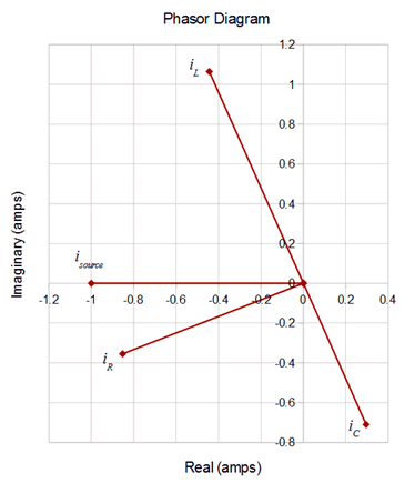
Now for the sneaky bit. In case you didn't notice, the components in this circuit are identical to those of Figure $\PageIndex{8}$ with the exception of the source. As a consequence, the phase angles and magnitudes of the branch currents through the three components will remain unchanged relative to each other. Due to the change in both magnitude and direction of the source, the entire phasor plot has been rotated clockwise by 154.7 degrees and all of the magnitudes have been lengthened by the ratio of the voltages $(9.231 / 2)$. This is perhaps easiest to see by focusing on the vector for $i_{source}$ in Figure $\PageIndex{9}$. Rotate that vector clockwise, along with every other vector, until $i_{source}$ lines up with the negative real axis. The result is the plot of Figure $\PageIndex{15}$, albeit with newly lengthened magnitudes.

If a parallel circuit contains multiple current sources, they may be added together (a vector sum, of course) to generate an equivalent single current source. The analysis then proceeds as before. This is demonstrated in the following example.

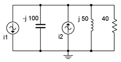
Example $\PageIndex{6}$

For the circuit of Figure $\PageIndex{16}$, determine the currents through the capacitor, inductor and resistor, and also determine the system voltage. $i_1$ is $0.5\angle 0^{\circ}$ amps and $i_2$ is $3\angle 45^{\circ}$ amps.

Figure $\PageIndex{16}$: Circuit for Example $\PageIndex{6}$.

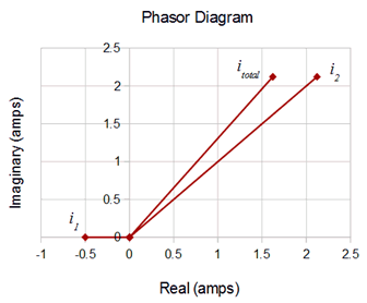
The first step here is to determine the effective current driving the circuit. If we treat the top node as positive, $i_2$ is entering (positive) while $i_1$ is exiting (negative). The combination is:

$$i_{total} = i_1 + i_2 \nonumber$$

$$i_{total} = −0.5\angle 0^{\circ} A +3\angle 45^{\circ} A \nonumber$$

$$i_{total} = 2.67\angle 52.6^{\circ} A \nonumber$$

This current has the same reference direction as source two. A phasor diagram of the process is illustrated in Figure $\PageIndex{17}$ to help visualize the vector addition.

Figure $\PageIndex{17}$: Phasor diagram of the combined current sources for the circuit for Example $\PageIndex{6}$.

The next step is to find the combined impedance so that we can find the applied voltage.

$$Z_{total} = \frac{1}{\frac{1}{Z_1} + \frac{1}{Z_2} + \frac{1}{Z_3}} \nonumber$$

$$Z_{total} = \frac{1}{\frac{1}{− j 100 \Omega} + \frac{1}{j 50\Omega} + \frac{1}{40 \Omega}} \nonumber$$

$$Z_{total} = 37.14\angle 21.8^{\circ} \Omega \nonumber$$

$$v = i_{source} \times Z_{total} \nonumber$$

$$v = 2.67\angle 52.6^{\circ} A\times 37.14\angle 21.8^{\circ} \nonumber$$

$$v \approx 99.16\angle 74.4^{\circ} V \nonumber$$

We now apply Ohm's law to each of the components to determine the branch currents.

$$i_C = \frac{v}{X_C} \nonumber$$

$$i_C = \frac{99.16\angle 74.4^{\circ} V}{100\angle −90^{\circ} \Omega} \nonumber$$

$$i_C \approx 0.9916\angle 164.4^{\circ} A \nonumber$$

$$i_L = \frac{v}{X_L} \nonumber$$

$$i_L = \frac{99.16\angle 74.4^{\circ} V}{50 \angle 90^{\circ} \Omega} \nonumber$$

$$i_L = 1.983\angle −15.6^{\circ} A \nonumber$$

$$i_R = \frac{v}{R} \nonumber$$

$$i_R = \frac{99.16\angle 74.4^{\circ} V}{40\angle 0^{\circ} \Omega} \nonumber$$

$$i_R = 2.479\angle 74.4 ^{\circ} A \nonumber$$

The sum of these three currents is approximately $2.67\angle 52.6^{\circ}$ amps. This balances the net entering current from the two sources, verifying KVL.