3.5.3: Transistor I-V Characteristics

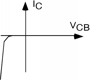
Let's now take a look at some current-voltage relationships for the bipolar transistor. In the absence of any voltage or current on the emitter-base junction, if we were to make a plot of \(I_{C}\) as a function of \(V_{\text{CB}}\), it would look something like Figure \(\PageIndex{1}\). Check back with the voltage convention in the figures on the structure and forward active biasing of a bipolar transistor to make sure you agree with what I drew. All we've got here is a PN junction or diode. It just happens to be biased in a reverse direction, so it conducts when \(V_{\text{CB}}\) $V_{\mathrm{CB}}$is negative and not when \(V_{\text{CB}}\) is positive. Thus, all we need to do is draw a diode curve, but upside down!

Figure \(\PageIndex{1}\): I-V graph for the collector-base terminals of the bipolar transistor

What happens if we now also have some bias applied to the emitter-base junction? As we saw, so long as the base-collector junction is reverse biased, almost all of the collector current consists of electrons which have been injected into the base by the emitter, diffuse across the base region, and then fall down the base-collector junction. The rate at which electrons fall down the junction does not depend on how large a drop there is (e.g. how big \(V_{\text{CB}}\) is). The only thing that matters, so far as the collector current is concerned, is how fast electrons are being injected into the base region, which is, of course, determined by the emitter current \(I_{E}\). Thus for several different values of emitter current, \(I_{E_{1}}\), \(I_{E_{2}}\), and \(I_{E_{3}}\), we might see something like Figure \(\PageIndex{2}\).

Figure \(\PageIndex{2}\): Common base characteristics of the bipolar transistor

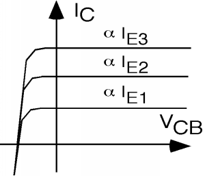
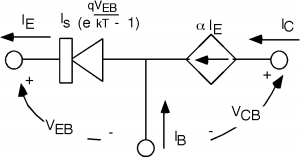
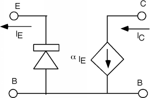
In the first quadrant, which is in the "forward active bias mode," the output from the collector terminal looks more or less like a current source; that is, \(I_{C}\) is a constant, regardless of what \(V_{\text{CB}}\) is. Note however, that we must use a controlled source, in this case, a current-controlled current source, since \(I_{C}\) depends on what \(I_{E}\) happens to be. Obviously, looking in the (forward biased) emitter-base terminal, we see the usual p-n junction. Thus, if we were interested in building a "model" of this device, we might come up with something like Figure \(\PageIndex{3}\). Note that the base terminal is common to both inputs. Since we would actually like to think of the transistor as a two-port device (with an input and an output) the model for the transistor is often drawn as shown in Figure \(\PageIndex{4}\).

Figure \(\PageIndex{3}\): Model for the common base transistor

Figure \(\PageIndex{4}\): Re-drawn common base transistor

The only drawback with what we have so far is that except in some specialized high-frequency circuits, the bipolar transistor is very rarely used in the common base configuration. Most of the time, you will see it in either the common emitter configuration (Figure \(\PageIndex{5}\)), or the common collector configuration. The common emitter is probably the way the transistor is most often used.

Figure \(\PageIndex{5}\): Configuration for the common emitter circuit

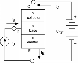
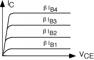
Note that we have a current source driving the base, and we have applied just one battery all the way from the collector to the emitter. The battery now has to do two things: a) It has to provide reverse bias for the base-collector junction and b) it has to provide forward bias for the base emitter junction. For this reason, the \(I_{C}\) as a function of \(V_{\text{CE}}\) curves look a little different now. It is now necessary for \(V_{\text{CE}}\) to become slightly positive in order to get the transistor into its active mode. The other difference, of course, is that the collector current is now shown as being \(\beta I_{B}\), the base current, instead of \(\alpha I_{E}\), the emitter current.

Figure \(\PageIndex{6}\): Common emitter characteristic curves for the transistor