3.5: Problems

Exercise \(\PageIndex{1}\) Airfoils

1. In a wind tunnel experiment it has been measured the distribution of pressures over a symmetric airfoil for an angle of attack of \(14^{\circ}\). The distribution of coefficient of pressures at the intrados, \(C_{pl}\), and extrados, \(C_{pE}\), of the airfoil can be respectively approximated by the following functions:
   \[C_{pl} (x) = \begin{cases} 1 - 2 \tfrac{x}{c}, \ \ \ \ \ \ & 0 \le x \le \tfrac{c}{4}, \\ \tfrac{2}{3} (1 - \tfrac{x}{c} ) \ \ \ \ \ \ & \tfrac{c}{4} \le x \le c; \end{cases}\nonumber\]
   \[C_{pE} (x) = \begin{cases} - 12 \tfrac{x}{c}, \ \ \ \ \ \ & 0 \le x \le \tfrac{c}{4}, \\ 4 (-1 + \tfrac{x}{c} ) \ \ \ \ \ \ & \tfrac{c}{4} \le x \le c. \end{cases}\nonumber\]
   (a) Draw the curve that represents the distribution of pressures.
   (b) Considering a chord \(c = 1\) m, obtain the coefficient of lift of the airfoil.
   (c) Calculate the slope of the characteristic curve \(c_l (\alpha)\).
2. Based on such airfoil as cross section, we build a rectangular wing with a wingspan of \(b = 20\) m and constant chord \(c = 1\) m. The distribution of the coefficient of lift along the wingspan of the wing (\(y\) axis) for an anglee of attack \(\alpha = 14^{\circ}\) is approximated by the following parabolic function:
   \[c_l (y) = 1.25 - 5 (\dfrac{y}{b})^2, - \dfrac{b}{2} \le y \le \dfrac{b}{2}.\nonumber\]
   (a) Draw the curve \(c_l (y)\).
   (b) Calculate the coefficient of lift of the wing.

Answer

1. 
   (a) The curve is as follows:
   
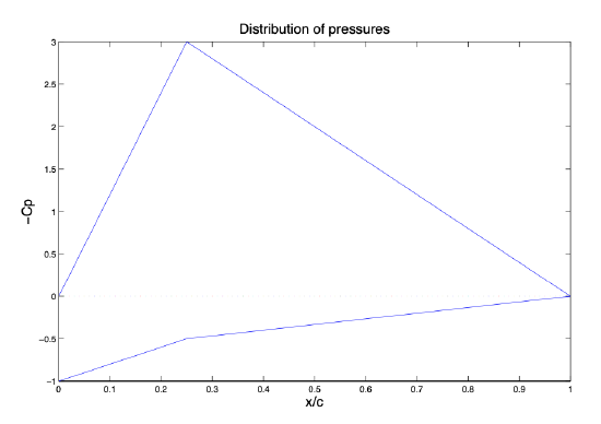
   Figure 3.28: Distribution of the coefficient of pressures.
   (b) The coefficient of lift for the airfoil for \(\alpha = 14^{\circ}\) can be calculated as follows:
   \[c_l = \dfrac{1}{c} \int_{x_{le}}^{x_{te}} (c_{pl} (x) - c_{pE} (x)) dx,\label{eq3.5.1}\]
   In this case, with \(c = 1\) and the given distributions of pressures of Intrados and extrados, Equation (\(\ref{eq3.5.1}\)) becomes:
   \[c_l = \dfrac{1}{c} \left [ \int_{0}^{1/4} ((1 - 2x) - (-12x)) dx + \int_{1/4}^{1} (2/3 (1 - x) - 4(-1 + x)) dx \right ] = 1.875. \nonumber\]
   (c) The characteristic curve is given by:
   \[c_l = c_{l_0} + c_{l_{\alpha}} \alpha.\nonumber\]
   Since the airfoil is symmetric: \(c_{l_0} = 0\). Therefore \(c_{l_{\alpha}} = \tfrac{c_l}{\alpha} = \tfrac{1.875 \cdot 360}{14 \cdot 2\pi} = 7.16 \ 1/rad\).
2. 
   (a) The curve is as follows:
   
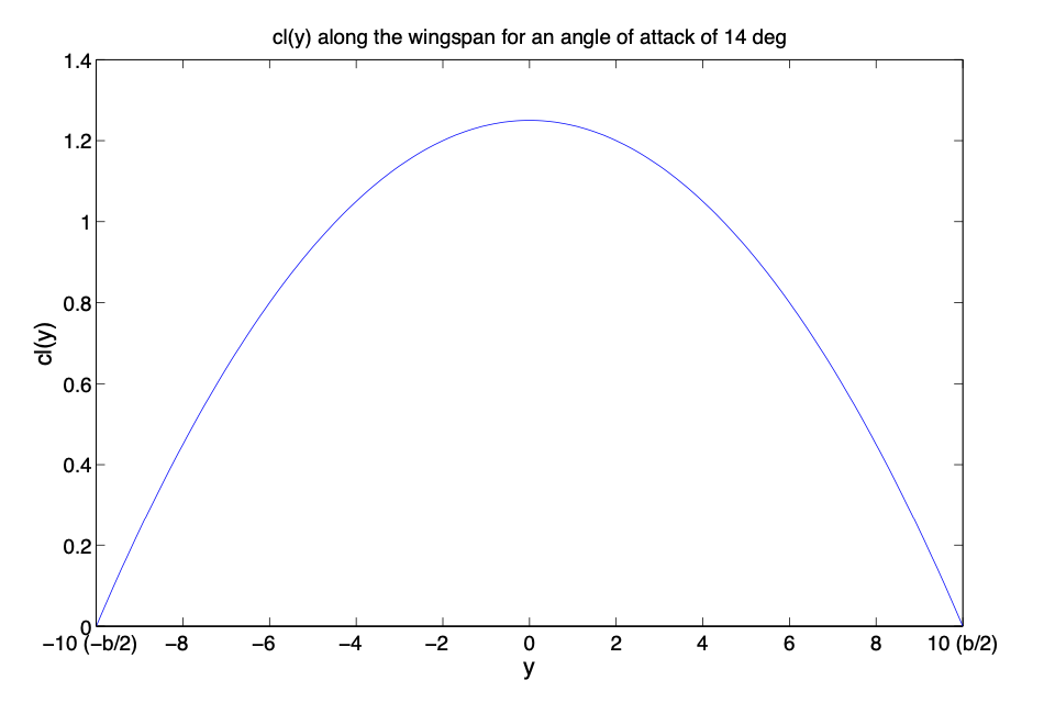
   Figure 3.29: Coefficient of lift along the wingspan.
   (b) The coefficient of lift for the wing for \(\alpha = 14^{\circ}\) can be calculated as follows:
   \[C_L = \dfrac{1}{S_w} \int_{-b/2}^{b/2} c(y) c_l (y) dy.\label{eq3.5.2}\]
   Substituting in Equation (\(\ref{eq3.5.2}\)) considering \(c(y) = 1\) and \(b = 20\):
   \[C_L = \dfrac{1}{20} \int_{-10}^{10} \left (1.25 - 5 (\dfrac{y}{20})^2 \right ) dy = 0.83.\nonumber\]

Exercise \(\PageIndex{2}\) Airfoils

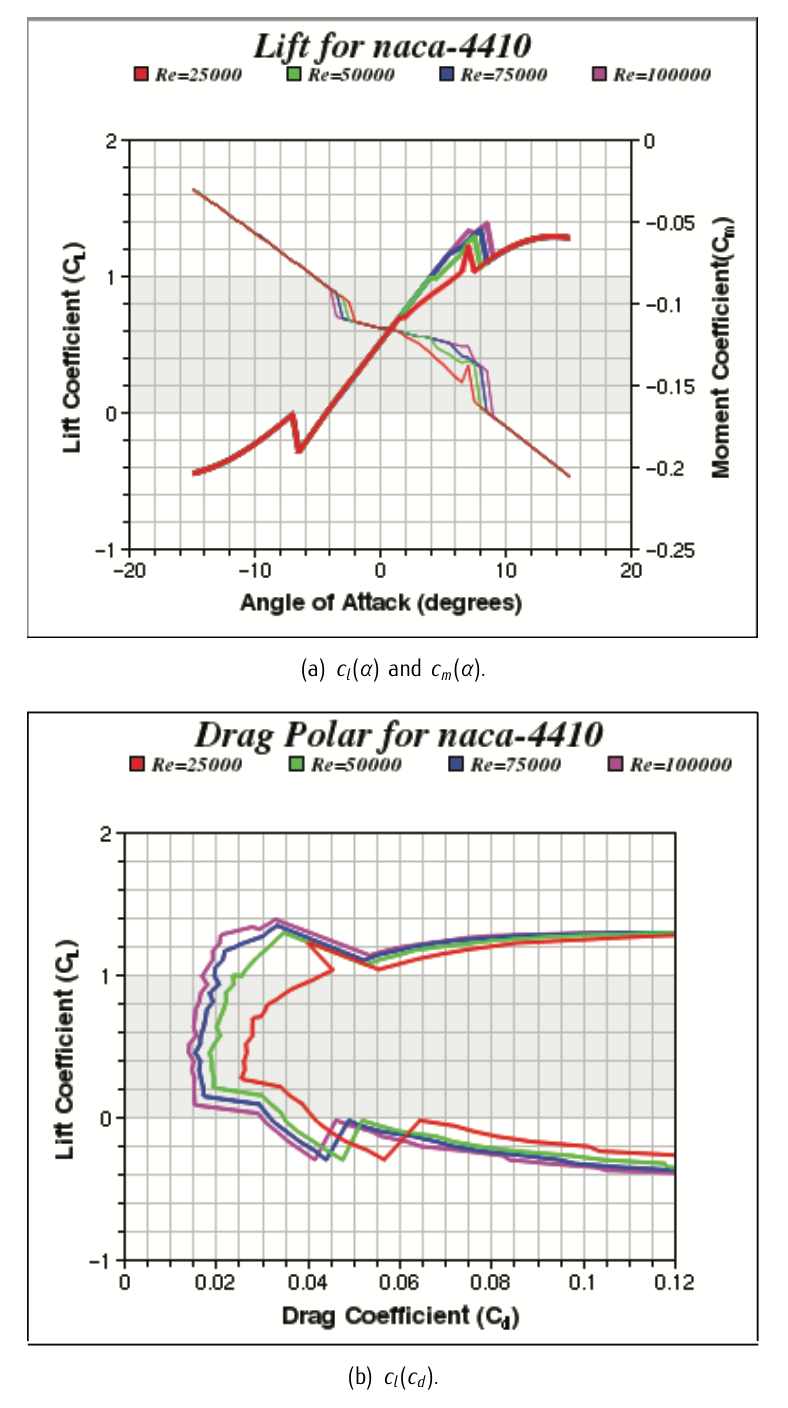
Figure 3.30: Characteristic curves of a NACA 4410 airfoil.

We want to know the aerodynamic characteristics of a NACA-4410 airfoil for a Reynolds number \(\text{Re} = 100000\). Experimental results gave the characteristic curves shown in Figure 3.30.

Calculate:

1. The expression of the lift curve in the linear range in the form: \(c_l = c_{l0} + c_{l\alpha} \alpha\).
2. The expression of the parabolic polar of the airfoil in the form: \(c_d = c_{d0} + b_{c_l} + kc_l^2.\)
3. the angle of attack and the coefficient of lift corresponding to the minimum coefficient of drag.
4. The angle of attack, the coefficient of lift and the coefficient of drag corresponding to the maximum aerodynamic efficiency.
5. The values of the aerodynamic forces per unity of longitude that the model with chord \(c= 2\) m would produce in the wind tunnel experiments with an angle of attack of \(\alpha = 3^{\circ}\) and incident current with Mach number \(M = 0.3\). Consider ISA conditions at an altitude of \(h = 1000\) m.

Answer

We want to approximate the experimental data given in Figure 3.30, respectively to a straight line and a parabolic curve. Therefore, to univocally define such curves, we must choose:

• Two pair of points (\(c_l, \alpha\)) of the \(c_l (\alpha)\) curve in Figure 3.30.a.
• Three pair of points (\(c_l, c_d\)) of the \(c_l (c_d)\) curve in Figure 3.30.b.

According to Figure 3.30 For \(\text{Re} = 100000\) we choose (any other combination properly chosen must work):

\(c_l\)	\(\alpha\)
0.5	\(0^{\circ}\)
1	\(4^{\circ}\)

Table 3.3: Date obtained from Figure 3.30.a.

\(c_l\)	\(c_d\)
0	0.03
1	0.0175
1.4	0.0325

Table 3.4: Data obtained from Figure 3.30.b.

1. The expression ofthe lift curve in the linear range in the form: \(c_l = c_{l0} + c_{l\alpha} \alpha\):
   With the data in Table 3.3:
   \[c_{l0} = 0.5;\]
   \[c_{l\alpha} = 7.16 \cdot 1/rad.\]
   The required curve yields then:
   \[c_l = 0.5 + 7.16 \alpha [\alpha \ in \ rad]\label{eq3.5.5}\]
2. The expression of the parabolic polar of the airfoil in the form: \(c_d = c_{d0} + bc_l + kc_l^2\):
   With the data in Table 3.4 we have a system of three equations with three unkowns that is to be solved. It yields:
   \[c_{d0} = 0.03;\]
   \[b = -0.048;\]
   \[k = 0.0357.\]
   The expression of the parabolic polar yields:
   \[c_d = 0.03 - 0.048 c_l + 0.0357 c_l^2.\label{eq3.5.9}\]
3. The angle of attack and the coefficient of lift corresponding to the minimum coefficient of drag:
   In order to do so, we seek the minimum of the parabolic curve:
   \[\dfrac{dc_l}{dc_d} = 0 = b + 2 \cdot kc_l.\]
   Substituting in Equation (\(\ref{eq3.5.9}\)):
   \[\dfrac{dc_l}{dc_d} = 0 = -0.048 + 2 \cdot 0.0357 c_l \to (c_l)_{c_{d_{\min}}} = 0.672.\]
   Substituting \((c_l)_{c_{d_{\min}}}\) in Equation (\(\ref{eq3.5.5}\)), we obtain:
   \[(\alpha)_{c_{d_{\min}}} = 0.024\ rad (1.378^{\circ}).\nonumber\]
4. The angle of attack, the coefficient of lift and the coefficient of drag corresponding to the maximum aerodynamic efficiency:
   The aerodynamic efficiency is defined as:
   \[E = \dfrac{l}{d} = \dfrac{c_l}{c_d}.\label{eq3.5.12}\]
   Substituting the parabolic polar curve in Equation (\(\ref{eq3.5.12}\)), we obtain:
   \[E = \dfrac{c_l}{c_{d0} + bc_l + kc_l^2}.\]
   In order to seek the values corresponding to the maximum aerodynamic efficiency, one must derivate and make it equal to zero, that is:
   \[\dfrac{dE}{dc_l} = 0 = \dfrac{c_{d0} - kc_l^2}{(c_{d0} + bc_l + kc_l^2)^2} \to (c_l)_{E_{\max}} = \sqrt{\dfrac{c_{d0}}{k}}.\]
   Substituting according to the values previously obtained (\(c_{d0} = 0.03, k = 0.0357\)): \((c_l)_{E_{\max}} = 0.91\). Substituting in Equation (\(\ref{eq3.5.5}\)) and Equation (\(\ref{eq3.5.9}\)), we obtain:
   \(\bullet (\alpha)_{E_{\max}} = 0.058\ rad\ (3.33^{\circ});\)
   \(\bullet (c_d)_{E_{\max}} = 0.01588.\)
5. The values of the aerodynamic forces per unity of longitude that the model with chord \(c = 2\) m would produce in the wind tunnel experiments with an angle of attack of \(\alpha = 3^{\circ}\) and incident current with Mach number \(M = 0.3\):
   According to ISA:
   \(\bullet \rho (h = 1000) = 0.907\ kg/m^3\);
   \(\bullet a(h = 1000) = \sqrt{\gamma_{air} R (T_0 - \lambda h)} = 336.4\ m/s\);
   where a corresponds to the speed of sound, \(\gamma_{air} = 1.4, R = 287\ J/KgK, T_0 = 288.15\ k\) and \(\lambda = 6.5 \cdot 10^{-3}\).
   Since the experiment is intended to be at \(M = 0.3\):
   \[V = M \cdot a = 100.92\ m/s.\]
   Since the experiment is intended to be at \(\alpha = 3^{\circ}\), using Equation (\(\ref{eq3.5.5}\)) and Equation (\(\ref{eq3.5.9}\)):
   \[c_l = 0.87;\]
   \[c_d = 0.01526.\]
   Finally:
   \[l = c_l \dfrac{1}{2} \rho c V^2 = 8036.77\ N/m;\]
   \[d = c_d \dfrac{1}{2} \rho c V^2 = 140.96\ N/m.\]

Exercise \(\PageIndex{3}\) Wings

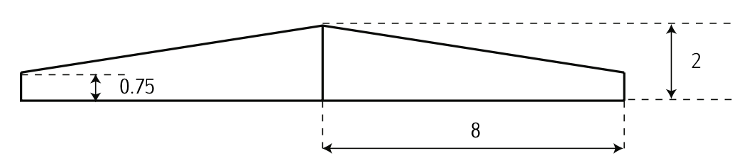
Figure 3.31: Plant-form of the wing (Dimensions in meters)

We want to analyze the aerodynamic performances of a trapezoidal wing with a plant-form as in Figure 3.31 and an efficiency factor of the wing of \(e = 0.96\). Moreover, we will employ a NACA 4415 airfoil with the following characteristics:

• \(c_l = 0.2 + 5.92 \alpha\).
• \(c_d = 6.4 \cdot 10^{-3} - 1.2 \cdot 10^{-3} c_l + 3.5 \cdot 10^{-3} c_l^2\).

Calculate:

1. The following parameters of the wing⁴: chord at the root; chord at the tip; mean chord; wing-spanl wet surface; enlargement.
2. The lift curve of the wing in the linear range.
3. The polar of the wing assuming that it can be calculated as \(C_D = C_{D_0} + C_{D_i} C_L^2\).
4. Calculate the optimal coefficient of lift, \(C_{L_{opt}}\), for the wing. Compare it with the airfoil's one.
5. Calculate the optimal coefficient of drag, \(C_{D_{opt}}\), for the wing. Compare it with the airfoil's one.
6. Maximum aerodynamic efficiency, \(E_{\max}\), for the wing. Compare it with the airfoils's one.
7. Discuss the differences observed in \(C_{L_{opt}}\), \(C_{D_{opt}}\), and \(E_{\max}\) between the wing and the airfoil.

Answer

1. Chord at the root; chord at the tip; mean chord; wing-span; wet surface; enlargement:

According the Figure 3.31:

The wing-span, \(b\), is \(b = 16\ m\). The chord at the ip, \(c_t\), is \(c_t = 0.75\ m\). The chord at the root, \(c_r\), is \(c_r = 2\ m\).

\[C_l = C_{l_0} + C_{l_{\alpha}} \alpha.\]

Therefore, with Equation (3.67) and Equation (3.68) in Equation (3.69), we have that:

We can also calculate the wet surface of the wing calculating twice the area of a tropezoid as follows:

\[S_w = 2 \left (\dfrac{(c_r + c_t)}{2} \dfrac{b}{2} \right ) = 22\ m^2.\nonumber\]

The mean chord, \(\bar{c}\), can be calculated as \(\bar{c} = \tfrac{S_w}{b} = 1.375\ m\); and the enlargement, \(A\), as \(A = \tfrac{b}{\bar{c}} = 11.63\).

2. Wing's lift curve:

The lift curve of a wing can be expressed as follows:

\[C_L = C_{L_0} + C_{L_{\alpha}} \alpha,\label{eq3.5.21}\]

and the slope of the wing's lift curve can be expressed related to the slope of the airfoil's lift curve as:

\[C_{L_{\alpha}} = \dfrac{C_{l_{\alpha}}}{1 + \tfrac{C_{t_{\alpha}}}{\pi A}} e = 4.89 \cdot 1/rad.\nonumber\]

In order to calculate the independent term of the wing’s lift curve, we must consider the fact that the zero-lift angle of attack of the wing coincides with the zero-lift angle of attack of the airfoil, that is:

\[\alpha (L = 0) = \alpha (l = 0).\label{eq3.5.22}\]

First, notice that the lift curve of an airfoil can be expressed as follows

\[C_l = C_{l_0} + C_{l_{\alpha}} \alpha.\label{eq3.5.23}\]

Therefore, with Equation (\(\ref{eq3.5.21}\)) and Equation (\(\ref{eq3.5.22}\)) in Equation (\(\ref{eq3.5.23}\)), we have that:

\[C_{L_0} = C_{l_0} \dfrac{C_{L_{\alpha}}}{C_{l_{\alpha}}} = 0.165.\nonumber\]

The required curve yields then:

\[C_L = 0.165 + 4.89 \alpha [\alpha \ in \ rad].\nonumber\]

3. The expression of the parabolic polar of the wing:

Notice first that the statement of the problem indicates that the polar should be in the following form:

\[C_D = C_{D0} + C_{D_i} C_L^2.\label{eq3.5.24}\]

For the calculation of the parabolic drag of the wing we can consider the parasite term approximately equal to the parasite term of the airfoil, that is, \(C_{D_0} = C_{d_0}\).

\(C_{D_i} = \dfrac{1}{\pi Ae} = 0.028.\nonumber\]

The expression of the parabolic polar yields then:

\[C_D = 0.0064 + 0.028 C_L^2.\label{eq3.5.25}\]

4. The optimal coefficient of lift, \(C_{L_{opt}}\), for the wing. Compare it with the airfoils's one.

The optimal coefficient of lift is that making the aerodynamic efficiency maximum. The aerodynamic efficiency is defined as:

\[E = \dfrac{L}{D} = \dfrac{C_L}{C_D}.\label{eq3.5.26}\]

Substituting the parabolic polar given in Equation (\(\ref{eq3.5.24}\)) in Equation (\(\ref{eq3.5.26}\)), we obtain:

\[E = \dfrac{C_L}{C_{D_0} + C_{D_i} C_L^2}.\]

In order to seek the values corresponding to the maximum aerodynamic efficiency, one must derivate and make it equal to zero, that is:

\[\dfrac{dE}{dC_L} = 0 = \dfrac{C_{D_0} - C_{D_i} C_L^2}{(C_{D_0} + C_{D_i} C_L^2)^2} \to (C_L)_{E_{\max}} = C_{L_{opt}} = \sqrt{\dfrac{C_{D_0}}{C_{D_i}}}.\label{eq3.5.28}\]

For the case of an airfoil, the aerodynamic efficiency is defined as:

\[E = \dfrac{1}{d} = \dfrac{c_l}{c_d}.\label{eq3.5.29}\]

Substituting the parabolic polar curve given in the statement in the form \(c_{d_0} + bc_l + kc_l^2\) in Equation (\(\ref{eq3.5.29}\)), we obtain:

\[E = \dfrac{c_l}{c_{d_0} + bc_l + kc_l^2}.\]

In order to seek the values corresponding to the maximum aerodynamic efficiency, one must derivate and make it equal to zero, that is:

\[\dfrac{dE}{dC_l} = 0 = \dfrac{c_{d_0} - kc_l^2}{(c_{d0} + bc_l + kc_l^2)^2} \to (C_l)_{E_{\max}} = (c_l)_{opt} = \sqrt{\dfrac{c_{d_0}}{k}}.\label{eq3.5.31}\]

According to the values previously obtained (\(C_{D_0} = 0.0064\) and \(C_{D_i} = 0.028\)) and the values given in the statement for the airfoil's polar (\(c_{d_0} = 0.0064\), \(k = 0.0035\)), substituting them in Equation (\(\ref{eq3.5.28}\)) and Equation (\(\ref{eq3.5.31}\)), respectively, we obtain:

• \((C_L)_{opt} = 0.478;\)
• \((c_l)_{opt} = 1.35.\)

5. The optimal coefficient of drag, \(C_{D_{opt}}\) for the wing. Compare it with the airfoils's one:

Once the optimal coefficient of lift has been obtained for both airfoil and wing, simply by substituting their values into both parabolic curves given respectively in the statement and in Equation (\(\ref{eq3.5.25}\)), we obtain:

\[C_{D_{opt}} = 0.0064 + 0.028 C_{l_{opt}}^2 = 0.01279.\nonumber\]

\[c_{d_{opt}} = 6.4 \cdot 10^{-3} - 1.2 \cdot 10^{-3} c_{l_{opt}} + 3.5 \cdot 10^{-3} c_{l_{opt}}^2 = 0.01115.\nonumber\]

6. Maximum aerodynamic efficiency \(E_{\max}\) for the wing. Compare it the the airfoils's one:

The maximum aerodynamic efficiency can be obtained as:

\[E_{\max_{wing}} = \dfrac{C_{L_{opt}}}{C_{D_{opt}}} = 37.\nonumber\]

\[E_{\max_{airfoil}} = \dfrac{c_{l_{opt}}}{c_{d_{opt}}} = 121.\nonumber\]

7. Discuss the differences observed in \(C_{L_{opt}}\), \(C_{D_{opt}}\) and \(E_{\max}\) between the wing and the airfoil.

According to the results it is straightforward to see that meanwhile the optimum coefficient of drag is similar for both airfoil and wing, the optimum coefficient of lift is approximately three times lower that the airfoil’s one. Obviously this results in an approximately three time lower efficiency for the wing when compared to the airfoil’s one.

What does it mean? A three dimensional aircraft made of \(2D\) airfoils generates much more drag than the \(2D\) airfoil in order to achieve a required lift. Therefore, we can not simply extrapolate the analysis of an airfoil to the wing.

Such loss of efficiency is due to the so-called induced drag by lift. The explanation behind this behavior is due to the difference of pressures between extrados and intrados. In particular, in the region close to the marginal border, there is an air current surrounding the marginal border which passes from the intrados, where the pressure is higher, to extrados, where the pressure is lower, giving rise to two vortexes, one in each border rotating clockwise and counterclockwise. This phenomena produces downstream a whirlwind trail.

The presence of this trail modifies the fluid filed and, in particular, modifies the velocity each wing airfoil "sees". In addition to the freestream velocity \(u_{\infty}\), a vertical induced velocity ui must be added (See Figure 3.23). The closer to the marginal border, the higher the induced velocity is. Therefore, the effective angle of attack of the airfoil is lower that the geometric angle, which explains both the reduction in the coefficient of lift (with respect to the bi-dimensional coefficient) and the appearance of and induced drag (See Figure 3.24).

Exercise \(\PageIndex{4}\) Airfoils and Wings

1. In a wind tunnel experiment we have measured teh distribution of pressures over a symmetric airfoil with angle of attack \(6^{\circ}\). The distributions of the coefficient of pressures for intrados \((C_{pl})\) and extrados \((C_{pE})\) can be approximated by the following functions:
   \[C_{pl} (x) = \begin{cases} 10 \tfrac{x}{c}, \ \ \ \ \ \ \ & 0 \le \tfrac{x}{c} \le \tfrac{1}{10}, \\ 2 - 10 \tfrac{x}{c}, \ \ \ \ \ & \tfrac{1}{10} \le \tfrac{x}{c} \le \tfrac{1}{5}; \\ 0, \ \ \ \ \ \ & \tfrac{1}{5} \le \tfrac{x}{c} \le 1. \end{cases}\nonumber\]
   \[C_{pE} (x) = \begin{cases} -15 \tfrac{x}{c}, \ \ \ \ \ \ \ & 0 \le \tfrac{x}{c} \le \tfrac{1}{5}, \\ \tfrac{-15}{4} (1 - \tfrac{x}{c}, \ \ \ \ \ & \tfrac{1}{5} \le \tfrac{x}{c} \le 1. \end{cases}\nonumber\]
   (a) Draw the curve \(-C_p (\tfrac{x}{c})\).
   (b) Considering \(c = 1 [m]\), calculate the coefficient of lift of the airfoil.
2. Based on the previous airfoil as transversal section, we want to design a rectangular wing with wing-span \(b\) and constant chord \(c = 1\ m\). The distribution of the coefficient of lift along the wing-span for angle of attack \(6^{\circ}\) can be approximated by the following function:
   \[c_l (y) = c_{l_{airfoil}} \cdot (1 - \dfrac{4}{A} \cdot (\dfrac{y}{b})^2), -\dfrac{b}{2} \le y \le \dfrac{b}{2},\nonumber\]
   being \(c_{l_{airfoil}}\) the coefficient of lift of the airfoil previously calculated and A the enlargement of the wing.
   (a) Calculate the coefficient of lift of the wing as a function of the enlargement \(A\).
   (b) Calculate the coefficient of lift of the wing for \(A = 1\), \(A = 8yA =\infty\).
   (c) Draw the distribtution of the coefficient of lift along the wing-span for \(A = 1, A = 8yA = \infty\). Discuss the results.

Answer

1. Airfoil:

(a) The curve is as follows:

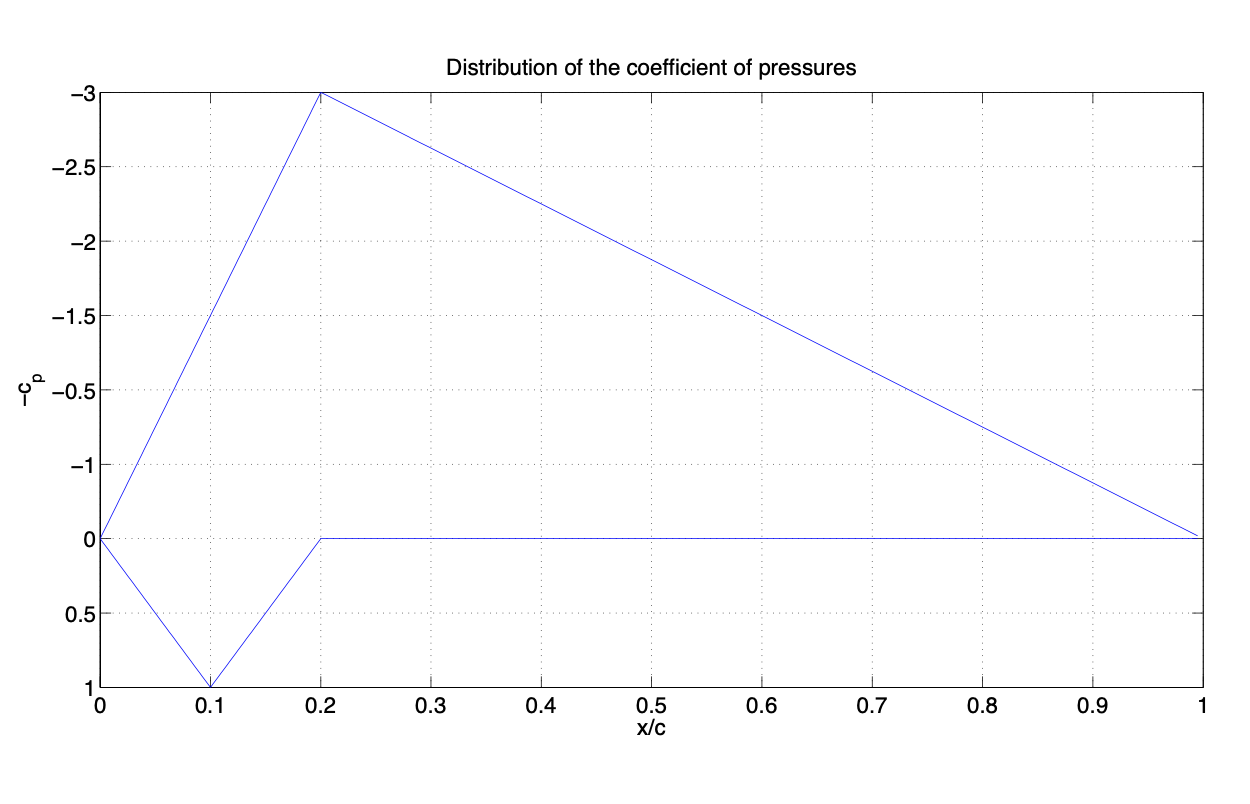
Figure 3.32: Distribution of the coefficient of pressures.

(b) The coefficient of lift of the airfoil for \(\alpha = 6^{\circ}\) can be calculate as follows:

\[c_l = \dfrac{1}{c} \int_{x_{le}}^{x_{te}} (c_{pl} (x) - c_{pE} (x)) dx.\label{eq3.5.32}\]

In this case, with \(c = 1\) and the given distributions of pressures of intrados and extrados, Equation (\(\ref{eq3.5.32}\)) becomes:

\[c_l = \dfrac{1}{c} \left [\int_{0}^{1/10} (10x) dx + \int_{1/10}^{1/5} (2 - 10x) dx + \int_{1/5}^{1} (0) dx - \int_{0}^{1/5} (-15x) dx - \int_{1/5}^{1} (-15/4 (1 - x)) dx \right ] = 1.6.\nonumber\]

2. Wing:

(a) The coefficient of lift for the wing for \(\alpha = 6^{\circ}\) can be calculated as follows:

\[C_L = \dfrac{1}{S_w} \int_{-b/2}^{b/2} c(y) c_l (y) dy.\label{eq3.5.33}\]

Substituting in Equation (\(\ref{eq3.5.33}\)) considering \(c(y) = 1\):

\[C_L = \dfrac{1}{b} \int_{-b/2}^{b/2} 1.6 \left (1 - \dfrac{4}{A} (\dfrac{y}{b})^2 \right ) dy = 1.6(1 - \dfrac{1}{3A}).\nonumber\]

(b) The values of \(C_L\) for the different enlargements are:

• \(A = 1 \to C_L = 1.06.\)
• \(A = 8 \to C_L = 1.53.\)
• \(A = \infty \to C_L = 1.6.\)

Considering, for instance, a wing-span \(b = 20\ m\), the curve is as follows:

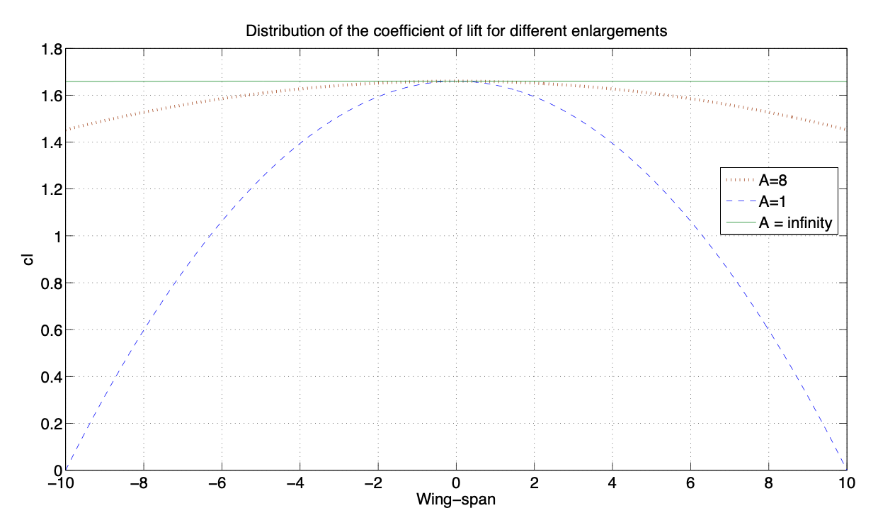
Figure 3.33: Coefficient of lift along the wingspan

(c) The discussion has to do with the differences in lift generation between finite and infinity wing.

It can be observed that if the enlargement is infinity the wing behaves as the bi-dimensional airfoil \(y (c_l(y)\) constant). On the other hand, if the enlargement is finite, \(c_l (y)\) shows a maximum in the root of the wing \((y = 0)\) and goes to zero in the tip of the wing \((y/c = A/2)\). As the enlargement decreases, the maximum \(c_l(y)\) also decreases.

The explanation behind this behavior is due to the difference of pressures between extrados and intrados. In particular, in the region close to the marginal border, there is an air current surrounding the marginal border which passes from the intrados, where the pressure is higher, to extrados, where the pressure is lower, giving rise to two vortexes, one in each border rotating clockwise and counterclockwise. This phenomena produces downstream a whirlwind trail.

The presence of this trail modifies the fluid field and, in particular, modifies the velocity each wing airfoil "sees". In addition to the freestream velocity, \(u_{\infty}\), a vertical induced velocity, \(u_i\), must be added (See Figure 3.23). The closer to the marginal border, the higher the induced velocity is. Therefore, the effective angle of attack of the airfoil is lower that the geometric angle, which explains both the reduction in the coefficient of lift (with respect to the bi-dimensional coefficient) and the fact that this reduction is higher when one gets closer to the marginal border.

Exercise \(\PageIndex{5}\) High-Lift devices

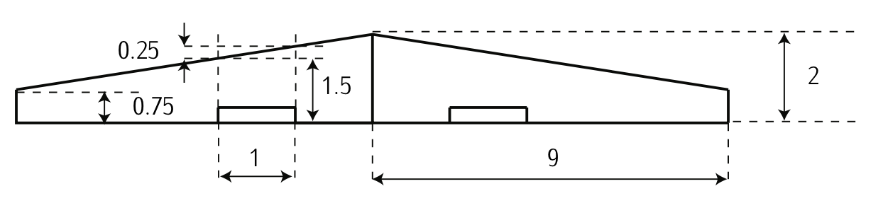
Figure 3.34: Plant-form of the wing (dimensions in meters).

We want to analyze the aerodynamic performances of a trapezoided wing with a plant-form as in Figure 3.34. The wing mounts two triple slotted Fowler flaps. The efficiency factor (Oswald factor) of the wing is \(e = 0.96\). The wing is build employing \(NACA\) 4415 airfoils with the following characteristics:

• ​​\(c_l = 0.2 + 5.92 \alpha\). (\(\alpha\) en radianes)
• \(c_d = 6.4 \cdot 10^{-3} - 1.2 \cdot 10^{-3} c_l + 3.5 \cdot 10^{-3} c_l^2\).

On regard of the effects of the Fowler flaps in the maximum coefficient of lift, it is known that:

• The increase of the maximum coefficient of lift of the airfoil (\(\Delta c_{l_{\max}}\)) can be approximated by the following expression:
  \[\Delta c_{l_{\max}} = 1.9 \dfrac{c'}{c},\label{eq3.5.34}\]
  being \(c\) the chord in the root and \(c'\) the extended chord (consider \(c' = 3\ [m]\)).
• The increase of the maximum coefficient of lift of the wing (\(\Delta C_{L_{\max}}\)) can be related to the increase of the maximum coefficient of lift of the airfoil (\(\Delta c_{l_{\max}}\)) by means of the following expression:
  \[\Delta C_{L_{\max}} = 0.92 \Delta c_{l_{\max}} \dfrac{S_{fw}}{S_w} \cos \wedge.\label{eq3.5.35}\]

Based on the data given in Figure 3.34, calculate:

(a) Chord in the root and tip of the wing. wing-span and enlargement. Wet wing surface (\(S_w\)) and surface wet by the flaps (\(S_{fw}\)). Aircraft swept (\(\wedge\)) measured from the leading edge.

Assuming a clean configuration (no flap deflection), typical of cruise conditions, and knowing also that the stall of the airfoil takes place at an angle of attack of \(15^{\circ}\):

(b) calculate the maximum coefficient of lift of the airfoil.

(c) calculate the expression of the lift curve of the wing in its linear range.

(d) calculate the maximum coefficient of lift of the wing (assume that the aircraft (wing) stalls also at an angle of attack of \(15^{\circ}\))

Assuming a configuration with flaps fully deflected, typical of a final approach, calculate:

(e) the maximum coefficient of lift of the wing.

It is known that the mass of the aircraft is \(4500\ kg\). For sea level \(ISA\) conditions and force due to gravity equal to \(9.81\ m/s^2\):

(f) calculate the stall speeds of the aircraft for both configurations (clean and full).

(g) compare and discuss the results.

Answer

(a). Chord at the root; chord at the tip; wing-span and enlargement; wing wet surface and flap wet surface; swept:

According to Figure 3.34:

• The wing-span, \(b\), is \(b = 18\ m\).
• The chord at the tip, \(c_t\), is \(c_t = 0.75\ m\).
• The chord at the root, \(c_r\), is \(c_r = 2\ m\).

We can also calculate the wet surface of the wing calculating twice the area of a trapezoid as follows:

\[S_w = 2 \left ( \dfrac{(c_r + c_t)}{2} \dfrac{b}{2} \right ) = 24.75\ m^2.\nonumber\]

In the same way, the flap wet surface \((S_{fw})\) can be calculated as follows:

\[S_{fw} = 2 \left ( 1 \cdot 1.5 + \dfrac{1}{2} 1 \cdot 0.25 \right ) = 3.25 \ m^2.\nonumber\]

The mean chord, \(\bar{c}\), can be calculated as \(\bar{c} = \tfrac{S_w}{b} = 1.375\ m\); and the enlargement, \(A\), as \(A = \tfrac{b}{\bar{c}} = 13.09\).

Finally, the swept of the wing (\(\wedge\)) measured from the leading edge is:

\[\wedge = \arctan (\dfrac{0.25}{1}) = 14^{\circ}.\nonumber\]

(b). \(c_{l_{\max}}\)

According to the expression given in the statement for the airfoil's lift curve: \(c_l = 0.2 + 5.92 \alpha\), and given that the airfoils stalls at \(\alpha = 15^{\circ}\), the maximum coefficient of lift will be given by the value of the coefficient of lift at the stall angle:

\[c_{l_{\max}} = 0.2 + 5.92 \cdot 15 \dfrac{2\pi}{360} = 1.74.\]

(c). Wing's lift curve:

The lift curve of a wing can be expressed as follows:

\[C_L = C_{L_0} + C_{L_{\alpha}} \alpha,\label{eq3.5.37}\]

and the slope of the wing’s lift curve can be expressed related to the slope of the airfoil’s lift curve as:

\[C_{L_{\alpha}} = \dfrac{C_{l_{\alpha}}}{1 + \tfrac{C_{l_{\alpha}}}{\pi A}} e = 4.96 \cdot 1/rad.\nonumber\]

In order to calculate the independent term of the wing’s lift curve, we must consider the fact that the zero-lift angle of attack of the wing coincides with the zero-lift angle of attack of the airfoil, that is:

\[\alpha (L = 0) = \alpha (l = 0).\label{eq3.5.38}\]

First, notice that the lift curve of an airfoil can be expressed as follows

\[C_l = C_{l_0} + C_{l_{\alpha}} \alpha.\label{eq3.5.39}\]

Therefore, with Equation (\(\ref{eq3.5.37}\)) and Equation (\(\ref{eq3.5.38}\)) in Equation (\(\ref{eq3.5.39}\)), we have that:

\[C_{L_0} = C_{l_0} \dfrac{C_{L_{\alpha}}}{C_{l_{\alpha}}} = 0.1678.\label{eq3.5.40}\]

The required curve yields then:

\[C_L = 0.1678 + 4.96 \alpha \ [\alpha \ in \ rad].\nonumber\]

(d). \(C_{L_{\max}}\) in clean configuration:

Given the expression in Equation (\(\ref{eq3.5.40}\)), and given that the aircraft (wing) stalls at \(\alpha = 15^{\circ}\), the maximum coefficient of lift will be given by:

\[C_{L_{\max}} = 0.1678 + 4.96 \cdot 15 \dfrac{2\pi}{360} = 1.466.\]

(e). \(C_{L_{\max}}\) in full configuration (with all flaps deflected):

In order to obtain the maximum coefficient of lift for full configuration \((C_{L_{\max}})\) we have that:

\[C_{L_{\max_f}} = C_{L_{\max}} + \Delta C_{L_{\max}}.\]

As it was given in the Equation (\(\ref{eq3.5.35}\)), \(\Delta C_{L_{\max}}\) can be expressed as:

\[\Delta C_{L_{\max}} = 0.92 \Delta c_{l_{\max}} \dfrac{S_{fw}}{S_w} \cos \wedge, \nonumber\]

where \(\wedge\), \(S_{fw}\), and \(S_w\) are already known and \(c_{l_{\max}}\) was given in Equation (\(\ref{eq3.5.34}\)). Therefore, \(\Delta C_{L_{\max}} = 0.334\).

\(C_{L_{\max_f}}\) yields then 1.8.

f. \(V_{stall}\):

Knowing that \(L = C_L \cdot \tfrac{1}{2} \rho S_w V^2\), that the flight can be considered to be equilibrated, i.e., \(L = m \cdot g\), and that the stall speed takes place when the coefficient of lift is maximum, we have that:

\[V_{stall} = \sqrt{\dfrac{m \cdot g}{\tfrac{1}{2} \rho S_w C_{L_{\max}}}} = 44.56 \ m/s.\nonumber\]

For the case of full configuration, we use \(C_{L_{\max_f}}\) and consider the wing-and-flap wet surface (notice that we are not including the chord extension in the wing wet surface). The stall velocity yields:

\[V_{stall_f} = \sqrt{\dfrac{m \cdot g}{\tfrac{1}{2} \rho (S_w + S_{fw}) C_{L_{\max_f}}}} = 37.8 \ m/s. \nonumber\]

g. Discussion:

High-lift devices are designed to increase the maximum coefficient of lift. By their deployment, they increase the aerodynamic chord and the camber of the airfoil, modifying thus the geometry of the airfoil so that the stall speed during specific phases of flight such as landing or take-off is reduced significantly, allowing to flight slower than in cruise.

Deploying high-lift devices also increases the drag coefficient of the aircraft. Therefore, for any given weight and airspeed, deflected flaps increase the drag force. Flaps increase the drag coefficient of an aircraft because of higher induced drag caused by the distorted span-wise lift distribution on the wing with flaps extended. Some devices increase the planform area of the wing and, for any given speed, this also increases the parasitic drag component of total drag.

By decreasing operating speed and increasing drag, high-lift device shorten takeoff and landing distances as well as improve climb rate. Therefore, these devices are fundamental during take-off (reduce the velocity at which the aircraft’s lifts equals aircraft’s weight), during the initial phase of climb (increases the rate of climb so that obstacles can be avoided) and landing (decrease the impact velocity and help braking the aircraft).

---

4. Based on the given data in Figure 3.31.