7.3: Problems

Exercise \(\PageIndex{1}\) Performances

Consider on Airbus A-320 with the following characteristics:

• \(m = 64\ tonnes.\)
• \(S_w = 122.6\ m^2.\)
• \(C_D = 0.024 + 0.0375 C_L^2\).

1. The aircraft starts an ascent maneuver with uniform velocity at 10.000 feet of altitue (3048 meters). At that flight level, the typical performances of the aircraft indicate a velocity with respect to air of 289 knots (\(148.67\ m/s\)) and a rate of climb (vertical velocity) of \(2760\ feet/min\) (\(14\ m/s\)). Assuming that \(\gamma \ll 1\), calculate:
   (a) The angle of ascent, \(\gamma\).
   (b) Required thrust at those conditions.
2. The aircraft reaches an altitude of \(11000\ m\), and performs a horizontal, steady, straight flight. Determine:
   (a) The velocity corresponding to the maximum aerodynamic efficiency.
3. The pilot switches off the engines and starts gliding at an altitude of \(11000\ m\). Calculate:
   (a) The minimum descent velocity (vertical velocity), and the corresponding angle of descent, \(\gamma_d\):

Answer

Besides the data given in the statement, the following data have been used:

• \(g = 9.81\ m/s^2\).
• \(R = 287\ J/(kgK)\).
• \(\alpha_T = 6.5 \cdot 10^{-3}\ K/m\).
• \(\rho_0 = 1.225\ kg/m^3\).
• \(T_0 = 288.15\ K\).
• \(ISA: \rho = \rho_0 (1 - \tfrac{\alpha_T h}{T_0})^{\tfrac{gR}{\alpha_T} - 1}\).

1. Uniform-ascent under the following flight conditions:
   \(\bullet\) \(h = 3048\ m\). Using \(ISA \to \rho = 0.904\ kg/m^3\).
   \(\bullet\) \(V = 148.67\ m/s\).
   \(\bullet\) \(h_e = 14\ m/s\).
   The system that governs the motion of the aircraft is:
   \[T = D + mg \sin \gamma;\]
   \[L = mg \cos \gamma;\]
   \[\dot{x}_e = V\cos \gamma;\]
   \[\dot{h}_e = V \sin \gamma.\]
   Assuming that \(\gamma \ll 1\), and thus that \(\cos \gamma \sim 1\) and \(\sin \gamma \sim \gamma\), System (B.1) becomes:
   \[T = D + mg \gamma;\label{eq7.3.5}\]
   \[L = mg;\label{eq7.3.6}\]
   \[\dot{x}_e = V;\]
   \[\dot{h}_e = V_{\gamma}.\label{eq7.3.8}\]
   (a) From Equation (\(\ref{eq7.3.8}\)), \(\gamma = \tfrac{\dot{h}_e}{V} = 0.094\ rad\ (5.39^{\circ})\).
   (b) From Equation (\(\ref{eq7.3.5}\)), \(T = D + mg\gamma\).
   \[D = C_D \dfrac{1}{2} \rho S_w V^2,\label{eq7.3.9}\]
   where \(C_D = 0.024 + 0.0375 C_L^2\), and \(\rho, S_w, V^2\) are known.
   \[C_L = \dfrac{L}{\tfrac{1}{2} \rho S_w V^2} = 0.512,\label{eq7.3.10}\]
   where, according to Equation (\(\ref{eq7.3.6}\)), \(L = mg\). With Equation (\(\ref{eq7.3.10}\)) in Equation (\(\ref{eq7.3.8}\)), \(D = 41398\ N\).
   Finally:
   \[T = D + mg\gamma = 100\ kN.\nonumber\]
2. Horizontal, steady, straight flight under the following flight conditions:
   \(\bullet\) \(h = 11000\ m\). Using \(ISA \to \rho = 0.3636\ kg/m^3\).
   \(\bullet\) The aerodynamic efficiency is maximum.
   The system that governs the motion of the aircraft is:
   \[T = D;\]
   \[L = mg \cos \gamma.\label{eq7.3.12}\]
   The maximum Efficiency is \(E_{\max} = \tfrac{1}{2\sqrt{C_{D_0} C_{D_i}}} = 16.66\).
   The optimal coefficient of lift is \(C_{L_{opt}} = \sqrt{\dfrac{C_{D_0}}{C_{D_i}}} = 0.8\).
   \[C_L = \dfrac{L}{\tfrac{1}{2} \rho S_w V^2} \to V = \dfrac{L}{\tfrac{1}{2} \rho S_w C_L} = 187\ m/s,\nonumber\]
   where, according to Equation (\(\ref{eq7.3.12}\)), \(L = mg\), and in order to fly with maximum efficiency: \(C_L = C_{L_{opt}}\).
3. Gliding under the following flight conditions:
   \(\bullet\) \(h = 11000\ m\). Using \(ISA \to \rho = 0.3636\ kg/m^3\).
   \(\bullet\) At the minimum descent velocity.
   The system that governs the motion of the aircraft is:
   \[D = mg\sin \gamma_d;\label{eq7.3.13}\]
   \[L = mg \cos \gamma_d;\label{eq7.3.14}\]
   \[\dot{x}_e = V \cos \gamma_d;\label{eq7.3.15}\]
   \[\dot{h}_{e_{des}} = V \sin \gamma_d.\label{eq7.3.16}\]
   Notice that \(\gamma_d = -\gamma\).
   Assuming that \(\gamma_d \ll 1\), and thus that \(\cos \gamma_d \sim 1\) and \(\sin \gamma_d \sim \gamma_d\), System (\(\ref{eq7.3.13}\), \(\ref{eq7.3.14}\), \(\ref{eq7.3.15}\), \(\ref{eq7.3.16}\)) becomes:
   \[D = mg \gamma_d;\label{eq7.3.17}\]
   \[L = mg;\label{eq7.3.18}\]
   \[\dot{x}_e = V;\]
   \[\dot{h}_{e_{des}} = V\gamma_d.\]
   In order to fly with maximum descent velocity \(\dot{h}_{e_{des}}\) must be maximum. Operating with Equation (\(\ref{eq7.3.17}\)) and Equation (\(\ref{eq7.3.18}\)), \(\gamma_d = \tfrac{D}{L}\).
   \[\dot{h}_{e_{des}} = V\gamma = V \dfrac{D}{L} = V \dfrac{(0.024 + 0.0375 C_L^2) \tfrac{1}{2} \rho S_w V^2}{C_L \tfrac{1}{2} \rho S_w V^2}.\label{eq7.3.21}\]
   knowing that \(C_L = \tfrac{L}{\tfrac{1}{2} \rho S_w V^2}\), where, according to Equation (\(\ref{eq7.3.18}\)), \(L = mg\), Equation (\(\ref{eq7.3.21}\)) becomes:
   \[\dot{h}_{e_{des}} = \dfrac{V}{mg} \left (0.024 \dfrac{1}{2} \rho S_w V^2 + \dfrac{0.0375 (mg)^2}{\tfrac{1}{2} \rho S_w V^2} \right ).\label{eq7.3.22}\]
   make \(\tfrac{\partial \dot{h}_{e_{des}}}{\partial V} = 0\).
   The velocity with respect to air so that the vertical velocity is minimum is:
   \[V = \sqrt[4]{\dfrac{4}{3} \dfrac{C_{D_i}}{C_{D_0}}} \sqrt{\dfrac{mg}{\rho S_w}} = 142.57\ m/s.\]
   Substituting \(V = 142.57\ m/s\) in Equation (\(\ref{eq7.3.22}\)), \(\dot{h}_{e_{des}} = 9.87\ m/s\).

Exercise \(\PageIndex{2}\) Runway performances

We want to estimate the take-off distance of an Airbus A-320 taking off at Madrid-Barajas airport. Such aircraft mounts two turbojets, which thrust can be estimated as: \(T = T_0 (1 - k\cdot V^2)\), where \(T\) is the thrust, \(T_0\) is the nominal thrust, \(k\) is a constant and \(V\) is the true airspeed.

Considering that:

• \(g \cdot (\tfrac{T_0}{m\cdot g} - \mu_r) = 1.31725 \tfrac{m}{s^2};\)
• \(\tfrac{\rho S(C_D - \mu_r C_L) + 2 \cdot T_0 \cdot k}{2 \cdot m} = 3.69 \cdot 19^{-5} \tfrac{m}{s^2};\)
• The velocity of take off is \(V_{TO} = 70\ m/s;\)

where \(g\) is the force due to gravity, \(m\) is the mass of the aircraft, \(\mu_r\) is the friction coefficient, \(\rho\) is the density of air, \(S\) is the wet surface area of the aircraft, \(C_D\) is the coefficient of lift⁹.

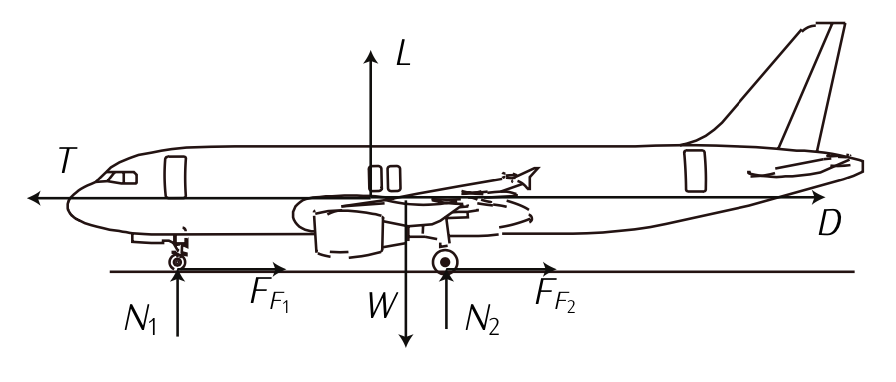
Figure 7.16: Forces during taking off

Calculate:

1. Take-off distance.

Answer

We apply the 2nd Newton's Law:

\[\sum F_z = 0;\label{eq7.3.24}\]

\[\sum F_x = m \dot{V}.\label{eq7.3.25}\]

Regarding Equation (\(\ref{eq7.3.24}\)), notice that while rolling on the ground, the aircraft is assumed to be under equilibrium along the vertical axis.

Looking at Figure 7.16, Equation (\(\ref{eq7.3.24}\))-(\(\ref{eq7.3.25}\)) become:

\[L + N - mg = 0;\label{eq7.3.26}\]

\[T - D - F_F = m \dot{V}.\]

being \(L\) the lift, \(N\) the normal force, \(mg\) the weight; \(T\) the trust, \(D\) the drag and \(F_F\) the total friction force.

It is well known that:

\[L = C_L \dfrac{1}{2} \rho S V^2;\label{eq7.3.28}\]

\[D = C_D \dfrac{1}{2} \rho S V^2.\label{eq7.3.29}\]

It is also well known that:

\[F_F = \mu_r N.\]

Equation (\(\ref{eq7.3.26}\)) states that: \(N = mg - L\). Therefore:

\[F_F = \mu_r (mg - L).\label{eq7.3.31}\]

Given that \(T = T_0 (1 - kV^2)\), with Equation (\(\ref{eq7.3.31}\)) and Equations  (\(\ref{eq7.3.28}\))-(\(\ref{eq7.3.29}\)), Equation (9.5.9) becomes:

\[\right (\dfrac{T_0}{m} -\mu_r g \right) + \dfrac{(\rho S (\mu_r C_L - C_D) - 2T_0 k)}{2m} V^2 = V.\label{eq7.3.32}\]

Now, we have to integrate Equation (\(\ref{eq7.3.32}\)).

In order to do so, as referred in the statement: \(T_0, m, \mu_r, g, \rho, S, C_L, C_D\) and \(k\) can be considered constant along the take off phase.

We have that:

\[\dfrac{dV}{dt} = \dfrac{dV}{dx} \dfrac{dx}{dt},\]

and knowing that \(\tfrac{dx}{dt} = V\), Equation (\(\ref{eq7.3.32}\)) becomes:

\[\dfrac{(\tfrac{T_0}{m} - \mu_r g) + \tfrac{(\rho S (\mu_r C_L - C_D) - 2T_0 k)}{2m} V^2}{V} = \dfrac{dV}{dx}.\label{eq7.3.34}\]

In order to simplify Equation (\(\ref{eq7.3.34}\)):

• \((\tfrac{T_0}{m} - \mu_r g) = g(\tfrac{T_0}{mg} - \mu_r) = A;\)
• \(\tfrac{(\rho S (\mu_r C_L - C_D) - 2T_0 k)}{2m} = B.\)

We proceed on integrating Equation (\(\ref{eq7.3.34}\)) between \(x = 0\) and \(x_{T0}\) (the distance of take off); \(V = 0\) (Assuming the maneuver starts with the aircraft at rest) and the velocity of take off that was given in the statement: \(V_{TO} = 70\ m/s\). It holds that:

\[\int_{0}^{x_{TO}} dx = \int_{0}^{V_{TO}} \dfrac{VdV}{A+ BV^2}.\]

Integrating:

\[\left [ x \right ]_{0}^{x_{TO}} = \left [ \dfrac{1}{2B} \ln (A + BV^2) \right ]_{0}^{V_{TO}}.\]

Substituting the upper and lower limits:

\[x_{TO} = \dfrac{1}{2B} \ln (1 + \dfrac{B}{A} V_{TO}^2).\]

Substituting the data given in the statement:

• \(A = 1.31725 \tfrac{m}{s^2};\)
• \(B = -3.69 \cdot 10^{-5} \tfrac{m}{s^2};\)
• \(V_{TO} = 70\ m/s.\)

The distance to take off is \(x_{TO} = 2000\ m\).

Exercise \(\PageIndex{3}\) Performances

An aircraft has the following characteristics:

• \(S_w = 130\ m^2\).
• \(b = 40\ m\).
• \(m = 70000\ kg\).
• \(T_{\max, av} (h = 0) = 120000\ N\) (Maximum available thrust at sea level).
• \(C_{D_0} = 0.02\).
• Oswald coefficient (wing efficiency coefficient): \(e = 0.9\).
• \(C_{L_{\max}} = 1.5\).

We can consider that the maximum thrust only varies with altitude as follows: \(T_{\max, av} (h) = T_{\max, av} (h = 0) \tfrac{\rho}{\rho_0}\). Consider standard atmosphere \(ISA\) and constant gravity \(g = 9.8\ m/s^2\). Determine:

1. The required thrust to fly at an altitude of \(h = 11000\ m\) with \(M_{\infty} = 0.7\) in horizontal, steady, straight flight.

2. The maximum velocity due to propulsive limitations of the aircraft and the corresponding Mach number in horizontal, steady, straight flight at \(h = 11000\).

3. The minimum velocity due to aerodynamic limitations (stall speed) in horizontal, steady, straight flight at an altitude of \(h = 11000\).

4. The theoretical ceiling (maximum altitude) in horizontal, steady, straight flight.

We want to perform a horizontal turn at an altitude of \(h = 11000\) with a load factor \(n = 2\), and with the velocity corresponding to the maximum aerodynamic efficiency in horizontal, steady, straight flight. Determine:

5. The required bank angle.

6. The radius of turn.

7. The required thrust. Can the aircraft perform the complete turn?

We want to perform a horizontal turn with the same load factor and the same radius as in the previous case, but at an altitude corresponding to the theoretical ceiling of the aircraft.

8. Can the aircraft perform such turn?

Answer

Besides that data given in the statement, the following data have been used:

• \(R = 287\ J/(kgK)\).
• \(\gamma_{air} = 1.4.\)
• \(\alpha_T = 6.5 \cdot 10^{-3} \ K/m\).
• \(\rho_0 = 1.225 \ kg/m^3\).
• \(T_0 = 288.15\ K\).
• \(ISA: \rho = \rho_0 (1 - \tfrac{\alpha_T h}{T_0})^{\tfrac{gR}{\alpha_T} - 1}.\)

1. Required Thrust to fly a horizontal, steady, straight flight under the following flight conditions:
   \(\bullet\) \(h = 11.000\ m\);
   \(\bullet\) \(M_{\infty} = 0.7.\)
   According to \(ISA\):
   \(\bullet\) \(\rho (h = 11000) = 0.364\ Kg/m^3\);
   \(\bullet\) \(a (h = 11000) = \sqrt{\gamma_{air} R (T_0 - \alpha_T h)} = 295.04\ m/s\).
   where a corresponds to the speed of sound.
   The system that governs the dynamics of the aircraft is:
   \[T = D;\label{eq7.3.37}\]
   \[L = mg;\label{eq7.3.38}\]
   being \(L\) the lift, \(mg\) the weight; \(T\) the trust and \(D\) the drag.
   It is well known that:
   \[L = C_L \dfrac{1}{2} \rho S_w V^2;\label{eq7.3.39}\]
   \[D = C_D \dfrac{1}{2} \rho S_w V^2.\label{eq7.3.40}\]
   It is also well known that the coefficient of drag can be expressed in a parabolic form as follows:
   \[C_D = C_{D_0} + C_{D_i} C_L^2,\label{eq7.3.41}\]
   where \(C_{D_0}\) is given in the statement and \(C_{D_i} = \tfrac{1}{\pi A e}\). The enlargement, \(A\), can be calculated as \(A = \tfrac{b^2}{S_w} = 12.30\) and therefore: \(C_{D_i} = 0.0287\).
   According to Equation (\(\ref{eq7.3.38}\)): \(L = 686000\ N\). The velocity of flight can be calculated as \(V = M_{\infty} a = 206.5\ m/s\). Once these values are obtained, with the values of density and wet surface, and entering in Equation (\(\ref{eq7.3.39}\)), we obtain that \(C_L = 0.68\).
   With the values of \(C_L\), \(C_{D_i}\), and \(C_{D_0}\), entering in Equation (\(\ref{eq7.3.41}\)) we obtain that \(C_D = 0.0332\).
   Looking now at Equation (\(\ref{eq7.3.37}\)) and using Equation (\(\ref{eq7.3.40}\)), we can state that the required thrust is as follows:
   \[T = C_D \dfrac{1}{2} \rho S_w V^2.\nonumber\]
   Since all values are known, the required thrust yields:
   \[T = 33567\ N.\nonumber\]
   Before moveing on, we should look wether the required thrust exceeds or not the maximum available thrust at the given altitude. In order to do that, it has been given that the maximum thrust only varies with altitude as follows:
   \[T_{\max, av} (h) = T_{\max, av} (h = 0) \dfrac{\rho}{\rho_0}.\]
   The maximum available thrust at \(h = 11000\) yields:
   \[T_{\max, av} (h = 11000) = 35657.14\ N.\label{eq7.3.43}\]
   Since \(T < T_{\max, av}\), the flight condition is flyable.
2. The maximum velocity due to propulsive limitations of the aircraft  and the corresponding Mach number is horizontal, steady, straight flight at \(h = 11000\):
   The maximum velocity due to propulsive limitation at the given altitude implies flying at the maximum available thrust that was obtained in Equation (\(\ref{eq7.3.43}\)).
   Looking again at Equation (\(\ref{eq7.3.37}\)) and using Equation (\(\ref{eq7.3.40}\)), we can state that:
   \[T_{\max, av} = C_D \dfrac{1}{2} \rho S_w V^2.\label{eq7.3.44}\]
   Using Equation (\(\ref{eq7.3.41}\)) and Equation (\(\ref{eq7.3.39}\)), and entering in Equation (\(\ref{eq7.3.44}\)) we have that:
   \[T_{\max, av} = \left ( C_{D_0} + C_{D_i} \left (\dfrac{L}{\tfrac{1}{2} \rho S_w V^2} \right )^2 \right ) \dfrac{1}{2} \rho S_w V^2.\label{eq7.3.45}\]
   Multiplying Equation (\(\ref{eq7.3.45}\)) by \(V^2\) we obtain a quadratic equation of the form:
   \[ax^2 + bx + c = 0.\]
   where \(x = V^2\), \(a = \tfrac{1}{2} \rho S_w C_{D_0}\), \(b = -T_{\max, av}\), and \(c = \dfrac{C_{D_i} L^2}{\tfrac{1}{2} \rho S_w}\).
   Solving the quadratic equation we obtain two different speeds at which the aircraft can fly given the maximum available thrust¹⁰. Those velocities yield:
   \[V_1 = 228\ m/s;\nonumber\]
   \[V_2 = 151\ m/s.\nonumber\]
   The maximum corresponds, obviously, to \(V_1\).
3. The minimum velocity due to aerodynamic limitations (stall speed) in horizontal, steady, straight flight at al altitde of \(h = 11000\).
   The stall speed takes place when the coefficient of lift is maximum, therefore, using Equation (\(\ref{eq7.3.39}\)), we have that:
   \[V_{stall} = \sqrt{\dfrac{L}{\tfrac{1}{2} \rho S_w C_{L_{\max}}}} = 139\ m/s.\nonumber\]
4. The theoretical ceiling (maximum altitude) in horizontal, steady, straight flight.
   In order to obtain the theoretical ceiling of the aircraft the maximum available thrust at that maximum altitude must coincide with the minimum required thrust to fly horizontal, steady, straight flight at that maximum altitude, that is:
   \[T_{\max, av} = T_{\min}.\label{eq7.3.47}\]
   Let us first obtain the minimum required thrust to fly horizontal, steady, straight flight. Multiplying and dividing by \(L\) in the second term of Equation (\(\ref{eq7.3.37}\)), and given that the aerodynamic efficiency is \(E = \tfrac{L}{D}\), we have that:
   \[T = \dfrac{D}{L} L = \dfrac{L}{E}.\]
   Since \(L\) is constant at those conditions of flight, the minimum required thrust occurs when the efficiency is maximum: \(T_{\min} \Leftrightarrow E_{\max}\).
   Let us now proceed deducing the maximum aerodynamic efficiency:
   The aerodynamic efficiency is defined as:
   \[E = \dfrac{L}{D} = \dfrac{C_L}{C_D}.\label{eq7.3.49}\]
   Substituting the parabolic polar curve given in Equation (\(\ref{eq7.3.41}\)) in Equation (\(\ref{eq7.3.49}\)), we obtain:
   \[E = \dfrac{C_L}{C_{D_0} + C_{D_i} C_L^2}.\label{eq7.3.50}\]
   In order to seek the values corresponding to the maximum aerodynamic efficiency, one must derivate and make it equal to zero, that is:
   \[\dfrac{dE}{dC_L} = 0 \dfrac{C_{D_0} - C_{D_i} C_L^2}{(C_{D_0} + C_{D_i} C_L^2)^2} \to (C_L)_{E_{\max}} = C_{L_{opt}} = \sqrt{\dfrac{C_{D_0}}{C_{D_i}}}.\label{eq7.3.51}\]
   Substituting the value of \(C_{L_{opt}}\) into Equation (\(\ref{eq7.3.50}\)) and simplifying we obtain that:
   \[E_{\max} = \dfrac{1}{2\sqrt{C_{D_0} C_{D_i}}}.\nonumber\]
   \(E_{\max}\) yields 20.86, and \(T_{\min} = 32870\ N\).
   According to Equation (\(\ref{eq7.3.43}\)) and based on Equation (\(\ref{eq7.3.47}\)) with \(T_{\min} = 32870\ N\), we have that:
   \[32870 = T_{\max, av} (h = 0) \dfrac{\rho}{\rho_0}.\nonumber\]
   Given that \(T_{\max, av} (h = 0)\) was given in the statement and \(\rho_0\) is known according to \(ISA\), we have that \(\rho = 0.335\ kg/m^3\).
   Since \(\rho_{h_{\max}} < \rho_{11000}\) we can easily deduce that the eiling belongs to the stratosphere. Using the \(ISA\) equation corresponding to the stratosphere we have that:
   \[\rho_{h_{\max}} = \rho_{11} \exp^{-\tfrac{g}{TR_{11}} (h_{\max} - h_{11})}.\label{eq7.3.52}\]
   where the subindex 11 corresponds to the values at the tropopause \((h = 11000\ m)\). Operating in Equation (\(\ref{eq7.3.52}\)), the ceiling yields \(h_{\max} = 11526\ m\).
5. The required bank angle:
   The equations governing the dynamics of the airplane in an horizontal turn are:
   \[T = D;\label{eq7.3.53}\]
   \[m V \dot{\chi} = L \sin \mu;\label{eq7.3.54}\]
   \[L \cos \mu = mg.\label{eq7.3.55}\]
   In a uniform (stationary) circular movement, it is well known that the tangential velocity is equal to the angular velocity (\(\dot{\chi}\)) multiplied by the radius o turn (\(R\)):
   \[V = \dot{\chi} R.\]
   Therefore, Sytem (\(\ref{eq7.3.53}\), \(\ref{eq7.3.54}\) and \(\ref{eq7.3.55}\)) can be rewritten as:
   \[T = D;\label{eq7.3.57}\]
   \[n \sin \mu = \dfrac{V^2}{gR};\label{eq7.3.58}\]
   \[n = \dfrac{1}{\cos \mu};\label{eq7.3.59}\]
   where \(n = \tfrac{L}{mg}\) is the load factor.
   Therefore, looking at Equation (\(\ref{eq7.3.59}\)), it is straightforward to determine that the bank angle of turn is \(\mu = 60^{\circ}\).
6. The radius of turn.
   First, we need to calculate the velocity corresponding to the maximum efficiency. As we have calculated before in Equation (\(\ref{eq7.3.51}\)), the coefficient of lift that generates maximum efficiency is the so-called optimal coefficient of lift, that is, \(C_{L_{opt}} = \sqrt{\dfrac{C_{D_0}}{C_{D_i}}} = 0.834\). The velocity yields then:
   \[V = \sqrt{\dfrac{L}{\tfrac{1}{2} \rho S_w C_{L_{opt}}}} = 186.4\ m/s.\nonumber\]
   Entering the Equation (\(\ref{eq7.3.58}\)) with \(\mu = 60\ [deg]\) and \(V = 186.4\ m/s\); \(R = 4093.8\ m\).
7. The required thrust.
   As exposed in Question 3, Equation (\(\ref{eq7.3.57}\)) can be expressed as:
   \[T = \dfrac{1}{2} \rho S_w V^2 C_{D_0} + \dfrac{L^2}{\tfrac{1}{2} \rho V^2 S_w} C_{D_i}.\nonumber\]
   Since all values are known: \(T = 32451\ N\)
   Since \(T \le T_{\max, av} (h = 110000)\), the aircraft can perform the turn.
8. We want to perform a horizontal turn with the same load factor and the same radius as the pervious case, but at an altitude corresponding to the thearetical ceiling of the aircraft. Can the aircraft perform the turn?
   If the load factor is the same, \(n = 2\), necessarily (according to Equation (\(\ref{eq7.3.59}\)) the bank angle is the same, \(\mu = 60^{\circ}\). Also, if the radius of turn is the same, \(R = 4093.8\ m\), necessarily (according to Equation (\(\ref{eq7.3.58}\)), the velocity of the turn must be the same as in the previous case, \(V = 186.4\ m/s\). Obviously, since the density will change according to the new altitude (\(\rho = 0.335\ kg/m^3\)), the turn will not be performed under maximum efficiency conditions.
   In order to know wheter the turn can be performed or not, we must compare the required thrust with the maximum available thrust at the ceiling altitude:
   \[T = \dfrac{1}{2} \rho S_w V^2 C_{D_0} + \dfrac{L^2}{\tfrac{1}{2} \rho V^2 S_w} C_{D_i} = 32983\ N.\nonumber\]
   \[T_{\max, av} (h = 11526) = T_{\max, av} (h = 0) \dfrac{\rho}{\rho_0} = 32816\ N.\nonumber\]
   Since \(T > T_{\max, av}\) at the ceiling, the turn can not be performed.

Exercise \(\PageIndex{4}\) Weights

Consider an Airbus A-320. Simplifying, we assume the wing of the aircraft is rectangle and it is composed on NACA 4415 airfoils. The characteristics of the NACA 4415 airfoils as follows:

• \(c_l = 0.2 + 5.92 \alpha\). (\(\alpha\) in radians).
• \(c_d = 6.4 \cdot 10^{-3} - 1.2 \cdot 10^{-3} c_l + 3.5 \cdot 10^{-3} c_l^2\).

Regarding the aircraft, the following data are known:

• Wing wet surface of 122.6 \([m^2]\).
• Wing-span of 34.1 \([m]\).
• Oswald efficiency factor of 0.95.
• Speific consumption per unity of thrust and time: \(\eta_j = 6.8 \cdot 10^{-5} [\tfrac{Kg}{N \cdot s}]\).

Calculate:

1. The lift of the wing in its linear range.
2. The drag polar curve, assuming it can be expressed as: \(C_D = C_{D_0} + C_{D_i} C_L^2\).
3. The optimal coefficient of lift of the wing, \(C_{L_{opt}}\). Compare it with the airfoil's one.

On regard of the characteristic weights of the aircraft, the following data are known:

• Operating empty weight \(OEW = 42.4\ [Ton]\).
• Maximum take-off weight \(MTOW = 77000 \cdot g\ [N]\)¹¹.
• Maximum fuel weight \(MFW = 29680 \cdot g\ [N]\).
• Maximum zero fuel weight \(MZFW = 59000 \cdot g\ [N]\).
• Moreoveer, the reserve fuel (\(RF\)) can be calculated as the 5% of the Trip Fuel (\(TF\)).

Calculate:

4. The Payload and Trip Fuel in the following cases:

(a) Initial weight equal to \(MTOW\) with the Maximum Payload \((MPL)\).
(b) Initial weight equal to \(MTOW\) with the Maximum Fuel Weight \((MFW)\).
(c) Initial weight equal to \(OEW\) plus \(MFW\).

Assuming that in cruise conditions the aircraft flies at a constant altitude of \(h = 11500\ [m]\), constant Mach number \(M = 0.78\), and maximum aerodynamic efficiency, considering \(ISA\) standard atmosphere, calculate:

5. Range and autonomy of the aircraft for the three initial weights pointed out above.

6. According to the obtained results, draw the payload-range diagram.

Answer

1. Wing's lift curve:
   The lift curve of a wing can be expressed as follows:
   \[C_L = C_{L_0} + C_{L_{\alpha}} \alpha,\label{eq7.3.60}\]
   and the slope of the wing's lift curve can be expressed related to the slope of the airfoil's lift curve as:
   \[C_{L_{\alpha}} = \dfrac{C_{l_{\alpha}}}{1 + \tfrac{C_{l_{\alpha}}}{\pi A}} e = 4.69 \cdot 1/rad.\nonumber\]
   In order to calculate the independent term of the wing's lift curve, we must consider the fact that the zero-lift angle of attack of the wing coincides with the zero-lift angle of attack of the airfoil, that is:
   \[\alpha (L = 0) = \alpha (l = 0).\label{eq7.3.61}\]
   First, notice that the lift curve of an airfoil can be expressed as follows
   \[C_l = C_{l_0} + C_{l_{\alpha}} \alpha.\label{eq7.3.62}\]
   Therefore, with Equation (\(\ref{eq7.3.60}\)) and Equation (\(\ref{eq7.3.61}\)) in Equation (\(\ref{eq7.3.62}\)), we have that:
   \[C_{L_0} = C_{l_0} \dfrac{C_{L_{\alpha}}}{C_{l_{\alpha}}} = 0.158.\nonumber\]
   The required curve yields then:
   \[C_L = 0.158 + 4.69 \alpha \ [\alpha \ in\ rad].\nonumber\]
2. The expression of the parabolic polar of the wing:
   Notice first that the statement of the problem indicates that the polar should be in the following form:
   \[C_D = C_{D_0} + C_{D_i} C_L^2.\label{eq7.3.63}\]
   For the calculation of the parabolic drag of the wing we can consider the parasite term approximately equal to the parasite term of the airfoil, that is, \(C_{D_0} = C_{d_0}\).
   The induced coefficient of drag can be calculated as follows:
   \[C_{D_i} = \dfrac{1}{\pi Ae} = 0.035.\nonumber\]
   The expression of the parabolic polar yields then:
   \[C_D = 0.0064 + 0.035 C_L^2.\]
3. The optimal coefficient of lift, \(C_{L_{opt}}\), for the wing. Compare it with the airfoils's one.
   The optimal coefficient of lift is that making the aerodynamic efficiency maximum. The aerodynamic efficiency is defined as:
   \[E = \dfrac{L}{D} = \dfrac{C_L}{C_D}.\label{eq7.3.65}\]
   Substituting the parabolic polar curve given in Equation (\(\ref{eq7.3.63}\)) in Equation (\(\ref{eq7.3.65}\)), we obtain:
   \[E = \dfrac{C_L}{C_{D_0} + C_{D_i} C_L^2}.\label{eq7.3.66}\]
   In order to seek the values corresponding to the maximum aerodynamic efficiency, one must derivate and make it equal to zero, that is:
   \[\dfrac{dE}{dC_L} = 0 = \dfrac{C_{D_0} - C_{D_i} C_L^2}{(C_{D_0} - C_{D_i} C_L^2)^2} \to (C_L)_{E_{\max}} = C_{L_{opt}} = \sqrt{\dfrac{C_{D_0}}{C_{D_i}}}.\label{eq7.3.67}\]
   For the case of an airfoil, the aerodynamic efficiency is defined as:
   \[E = \dfrac{l}{d} = \dfrac{c_l}{c_d}.\label{eq7.3.68}\]
   Substituting the parabolic polar curve given in the statement in the form \(c_{d_0} + bc_l + kc_l^2\) in Equation (\(\ref{eq7.3.68}\)), we obtain:
   \[E = \dfrac{c_l}{c_{d_0} + bc_l + kc_l^2}.\]
   In order to seek the values corresponding to the maximum aerodynamic efficiency, one must derivate and make it equal to zero, that is:
   \[\dfrac{dE}{dC_l} = 0 = \dfrac{c_{d_0} - kc_l^2}{(c_{d_0} + bc_l + kc_l^2)^2} \to (c_l)_{E_{\max}} = (c_l)_{opt} = \sqrt{\dfrac{c_{d_0}}{k}}.\label{eq7.3.70}\]
   According to the values previously obtained (\(C_{D_0} = 0.0064\) and \(C_{D_i} = 0.035\)) and the values given in the statement for the airfoil's polar (\(c_{d_0} = 0.0064\), \(k = 0.0035\)), substituting them in Equation (\(\ref{eq7.3.67}\)) and Equation (\(\ref{eq7.3.70}\)), respectively, we obtain:
   \(\bullet\) \((C_L)_{opt} = 0.42;\)
   \(\bullet\) \((c_l)_{opt} = 1.35.\)
4. Payload and Trip Fuel for case (a), (b), and (c):
   Before starting we the particular cases, it is necessary to point out that:
   \[TOW = OEW + PL + FW,\label{eq7.3.71}\]
   \[FW = TF + RF,\label{eq7.3.72}\]
   \[MZFW = OEW + MPL.\label{eq7.3.73}\]
   Moreover, according to the statement,
   \[RF = 0.05 \cdot TF.\]
   Based on the data given in the statement, and using Equation (\(\ref{eq7.3.73}\)):
   \[MPL = 16.6\ [Ton.].\]
   Case (a) Initial weight¹² \(\to\) \(MTOW\) with \(MPL\).
   Equation (\(\ref{eq7.3.71}\)) becomes:
   \[MTOW = OEW + MPL + TF + 0.05 \cdot TF,\label{eq7.3.76}\]
   Isolating in Equation (\(\ref{eq7.3.76}\)): \(TF = 17.14\ [Ton]\). The payload is equal to the maximum payload \(MPL\).
   Case (b) Initial weight \(\to\) \(MTOW\) with \(MFW\).
   Equation (\(\ref{eq7.3.71}\)) becomes:
   \[MTOW = OEW + PL + MFW,\label{eq7.3.77}\]
   Isolating in Equation (\(\ref{eq7.3.77}\)): \(PL = 4.92\ [Ton]\). In order to calculate the trip fuel, looking at Equation (\(\ref{eq7.3.72}\)), we have that 
   \[MFW = TF + RF = TF + 0.05 \cdot TF.\]
   Isolating, \(TF = 28.266\ [Ton.]\).
   Case (c) Initial weight \(\to\) \(OEW + MFW\).
   Equation (\(\ref{eq7.3.71}\)) becomes:
   \[TOW = OEW + MFW,\]
   That means \(PL = 0\), in order to calculate the trip fuel, we proceed exactly as in Case (b). Looking at Equation (\(\ref{eq7.3.72}\)), we have that
   \[MFW = TF + RF = TF + 0.05 \cdot TF.\]
   Isolating, \(TF = 28.266\ [Ton.]\)
5. Range and Endurance for cases (a), (b) and (c): Considering that the aircraft performs a linear, horizontal steady flight, we have that:
   \[L = mg;\label{eq7.3.81}\]
   \[T = D;\label{eq7.3.82}\]
   \[\dot{x} = V;\label{eq7.3.83}\]
   \[\dot{m} = -\eta T.\label{eq7.3.84}\]
   Since \(\dot{x} = \tfrac{dx}{dt}\), it is clear that the Range, \(R\), looking at Equation (\(\ref{eq7.3.83}\)), can be expressed as:
   \[R = \int_{t_i}^{t_f} V dt.\label{eq7.3.85}\]
   Now, since \(\dot{m} = \tfrac{dm}{dt} = -\eta T\), Equation (\(\ref{eq7.3.85}\)):
   \[R = \int_{m_i}^{m_f} -\dfrac{V}{\eta T} dm,\label{eq7.3.86}\]
   where \(m_i\) is the initial mass and \(m_f\) is the final mass.
   Using Equation (\(\ref{eq7.3.81}\)) and Equation (\(\ref{eq7.3.82}\)), Equation (\(\ref{eq7.3.86}\)) yields:
   \[R = \int_{m_i}^{m_f} - \dfrac{VE}{\eta g} \dfrac{dm}{m}.\]
   with \(E = \tfrac{L}{D}, V, \eta\), and \(g\) are constant values.
   Integrating:
   \[R = \dfrac{VE}{\eta g} \ln (\dfrac{m_i}{m_f}).\label{eq7.3.88}\]
   For the endurance, we operate analogously, integrating Equation (\(\ref{eq7.3.84}\)), which yields
   \[t = \int_{m_i}^{m_f} - \dfrac{1}{\eta T} dm.\label{eq7.3.89}\]
   Using Equation (\(\ref{eq7.3.81}\)) and (\(\ref{eq7.3.82}\)), (\(\ref{eq7.3.89}\)) yields:
   \[t = \int_{m_i}^{m_f} - \dfrac{E}{\eta g} \dfrac{dm}{m}.\]
   where again \(E = \tfrac{L}{D}\), \(\eta\) and \(g\) are constant values. Integrating:
   \[t = \dfrac{E}{\eta g} \ln (\dfrac{m_i}{m_f}).\label{eq7.3.91}\]
   Before calculating Range and Endurance for the three cases, we need to calculate the values of velocity and aerodynamic efficiency, which is maximum.
   The velocity can be expressed as \(V = M \cdot a\), where \(a\) is the speed of sound, that can be expressed as
   \[a = \sqrt{\gamma RT},\]
   where \(\gamma = 1.4\) is adiabatic coefficient of air, and \(R = 287\ J/KgK\) is the perfect gas constant. Notice that, using \(ISA\), the temperature at the stratosphere is constant, and thus \(T = 216.6\ K\).
   Substituting all terms, it yields \(v = 230.1\ [m/s]\).
   The aeerodynamic efficiency is maximum. Thus, substituting \(C_{L_{opt}}\) obtained in Equation (\(\ref{eq7.3.67}\)) into Equation (\(\ref{eq7.3.66}\)), it yields:
   \[E = \dfrac{1}{2\sqrt{C_{D_0} C_{D_i}}} = 33.4.\]
   Now, we should calculate the initial and final mass for of the three cases a), b), c). Notice that the final mass results from subtracting the trip fuel from the take-off mass:
   \[m_f = m_i - TF.\]
   Thus,
   (a) \(m_i = \dfrac{MTOW}{g} [Kg]\) and \(m_f = 59860\ [Kg]\).
   (b) \(m_i = \dfrac{MTOW}{g} [Kg]\) and \(m_f = 48734\ [Kg]\).
   (c) \(m_i = 72080 [Kg]\) and \(m_f = 43814\ [Kg]\).
   Substituting in Equation (\(\ref{eq7.3.88}\)) and Equation (\(\ref{eq7.3.91}\)), it yields:
   (a) \(R_a = 2900\ [Km]\) and \(t_a = 12600\ [s]\).
   (b) \(R_b = 5270\ [Km]\) and \(t_b = 22900\ [s]\).
   (c) \(R_c = 5736\ [Km]\) and \(t_c = 24928\ [s]\).
6. Payload-Range diagram cases (a), (b) and (c):
   
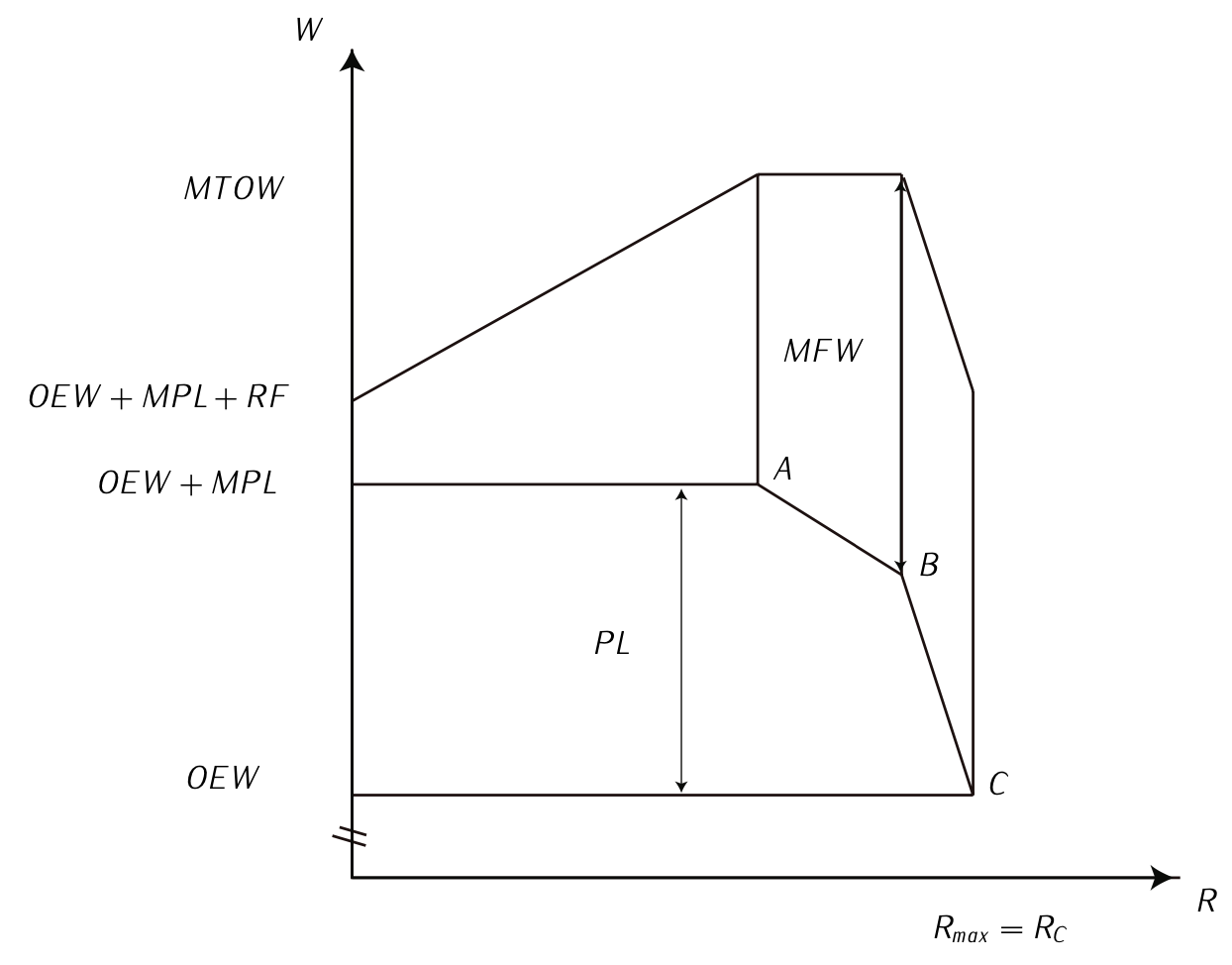
                                        Figure 7.17: Payload-range diagram

Exercise \(\PageIndex{5}\)

An aircraft has the following characteristics:

• \(S_w = 130\ m^2\).
• \(b = 40\ m\).
• \(m = 70000\ kg\).
• \(T_{\max, av, 0} = 130000\ N\) (Maximum available thrust at sea level).
• \(C_{D_0} = 0.02\).
• Oswald efficiency factor: \(e = 0.9\).

The maximum available thrust can be considered to vary according to the following law:

\[T_{\max, av} (h) = T_{\max, av, 0} \dfrac{\rho}{\rho_0}.\nonumber\]

Consider \(ISA\) atmosphere and constant gravity \(g = 9.8\ m/s^2\). Determine:

1. The required thrust to fly at an altitude of \(h = 11250\ m\) at \(M_{\infty} = 0.78\) in steady linear-horizontal flight.
2. The maximum speed of the aircraft due to propulsive limitations in steady linear-horizontal flight at an altitude of \(h = 11250\ m\).
3. The theoretical ceiling of the aircraft in steady linear-horizontal flight.

We want now to deteremine the surface of the horizontal stabilizer and as a design criterion we take the flight conditions of equilibrium at an altitude of \(h = 11250\ m\) & \(M_{\infty} = 0.78\). In those conditions, the coefficient of lift of the stabilizer is equal to 1.4. Moreover, we can assume that the distribution of lift of the wing can be reduced to a resultant force in the aerodynamic center (lift) and a pitching down moment with respect to the aerodynamic center equal to \(10000\ N \cdot m\). The distance between the aerodynamic center and the center of gravity (note that the aerodynamic center is closer to the nose of the aircraft) is \(x_{cg} = 2\ m\). The distance between the stabilizer and the center of gravity is \(l = 20\ m\).

4. Determine the surface of the horizontal stabilizer for those flight conditions.

Answer

Besides the data given in the statement, the following data have been used:

• \(R = 287\ J/(kgK)\).
• \(\gamma_{air} = 1.4\).
• \(T_{11} = 216.6\ K\).
• \(\rho_{11} = 0.36\ kg/m^3\).
• \(T_0 = 288.15\ K\).
• \(ISA: \rho = \rho_{11} \cdot e^{\tfrac{-gR}{T_{11}}} (h - 11000)\).

1. Required Thrust to fly a horizontal, steady, straight flight under the following flight conditions:
   \(\bullet\) \(h = 11.250\ m\).
   \(\bullet\) \(M_{\infty} = 0.78\).
   According to \(ISA\):
   \(\bullet\) \(\rho (h = 11250) = 0.3461\ Kg/m^3\).
   \(\bullet\) \(a (h = 11250) = \sqrt{\gamma_{air} R(T_{11})} = 295\ m/s\).
   where a corresponds to the speed of sound.
   The system that governs the dynamics of the aircraft is:
   \[T = D,\label{eq7.3.95}\]
   \[L = mg,\label{eq7.3.96}\]
   being \(L\) the lift, \(mg\) the weight; \(T\) the trust and \(D\) the drag.
   It is well known that:
   \[L = C_L \dfrac{1}{2} \rho S_w V^2;\label{eq7.3.97}\]
   \[D = C_D \dfrac{1}{2} \rho S_w V^2.\label{eq7.3.98}\]
   It is also well known that the coefficient of drag can be expressed in a prabolic form as follows:
   \[C_D = C_{D_0} + C_{D_i} C_L^2,\label{eq7.3.99}\]
   where \(C_{D_0}\) is given in the statement and \(C_{D_i} = \tfrac{1}{\pi Ae}\). The enlargement \(A\) can be calculated as \(A = \tfrac{b^2}{S_w} = 12.30\) and therefore: \(C_{D_i} = 0.0287\).
   According to Equation (\(\ref{eq7.3.96}\)): \(L = 686000\ N\). The velocity of flight can be calculated as \(V = M_{\infty} a = 230.1\ m/s\). Once these values are obtained, with the values of density and wet surface, and entering in Equation (\(\ref{eq7.3.97}\)), we obtain that \(C_L = 0.5795\).
   With the values of \(C_L, C_{D_i}\) and \(C_{D_0}\), entering in Equation (\(\ref{eq7.3.99}\)) we obtain that \(C_D = 0.0295\).
   Looking now at Equation (\(\ref{eq7.3.95}\)) and using Equation (\(\ref{eq7.3.98}\)), we can state that the required thrust is as follows:
   \[T = C_D \dfrac{1}{2} \rho S_w V^2.\nonumber\]
   Since all values are known, the required thrust yields:
   \[T = 35185\ N.\nonumber\]
   Before moving on, we should look wether the required thrust exceeds or not the maximum available thrust at the given altitude. In order to do that, it has been given that the maximum thrust only varies with altitude as follows:
   \[T_{\max, av} (h) = T_{\max, av, 0} \dfrac{\rho}{\rho_0}.\label{eq7.3.100}\]
   The maximum available thrust at \(h = 11250\) yields:
   \[T_{\max, av} (h = 11250) = 36729\ N.\label{eq7.3.101}\]
   Since \(T < T_{\max, av}\), the flight condition is flyable.
2. The maximum velocity due to propulsive limitations of the aircraft in horizontal, steady, straight flight at \(h = 11250\):
   The maximum velocity due to propulsive limitation at the given altitude implies flying at the maximum available thrust that was obtained in Equation (\(\ref{eq7.3.101}\)).
   Looking agian at Equation (\(\ref{eq7.3.95}\)) and using Equation (\(\ref{eq7.3.98}\)), we can state that:
   \[T_{\max, av} = C_D \dfrac{1}{2} \rho S_w V^2.\label{eq7.3.102}\]
   Using Equation (\(\ref{eq7.3.99}\)) and Equation (\(\ref{eq7.3.97}\)), and entering in Equation (\(\ref{eq7.3.102}\)) we have that:
   \[T_{\max, av} = \left (C_{D_0} + C_{D_i} \left (\dfrac{L}{\tfrac{1}{2} \rho S_w V^2} \right )^2 \right ) \dfrac{1}{2} \rho S_w V^2.\label{eq7.3.103}\]
   Multiplying Equation (\(\ref{eq7.3.103}\)) by \(V^2\) we obtain a quadratic equation of the form:
   \[ax^2 + bx + c = 0.\]
   where \(x = V^2\), \(a = \dfrac{1}{2} \rho S_w C_{D_0}, b = - T_{\max, av}\) and \(c = \dfrac{C_{D_i} L^2}{\tfrac{1}{2} \rho S_w}\).
   Solving the quadratic equation we obtain two different speeds at which the aircraft can fly given the maximum available thrust13. Those velocities yield:
   \[V_1 = 218\ m/s;\nonumber\]
   \[V_2 = 184.06\ m/s.\nonumber\]
   The maximum speeds corresponds, obviously, to \(V_1\).
3. The theoretical ceiling (maximum altitude) in horizontal, steady, straight flight.
   In order to obtain the theoretical ceiling of the aircraft the maximum available thrust at that maximum altitude must coincide with the minimum required thrust to fly horizontal, steady, straight flight at that maximum altitude, that is:
   \[T_{\max, av} = T_{\min}.\label{eq7.3.105}\]
   Let us first obtain the minimum required thrust to fly horizontal, steady, straight flight. Multiplying and dividing by \(L\) in the second term of Equation (\(\ref{eq7.3.95}\)), and given that the aerodynami efficiency is \(E = \tfrac{L}{D}\), we have that:
   \[T = \dfrac{D}{L} L = \dfrac{L}{E}.\]
   Since \(L\) is constant at those conditions of flight, the minimum required thrust occurs when the efficiency is maximum: \(T_{\min} \Leftrightarrow E_{\max}\).
   Let us now proceed deducing the maximum aerodynamic efficiency:
   The aerodynamic efficiency is defined as:
   \[E = \dfrac{L}{D} = \dfrac{C_L}{C_D}.\label{eq7.3.107}\]
   Substituting the parabolic polar curve gicen in Equation polar curve given in Equation (\(\ref{eq7.3.99}\)) in Equation (\(\ref{eq7.3.107}\)), we obtain:
   \[E = \dfrac{C_L}{C_{D_0} + C_{D_i} C_L^2}.\label{eq7.3.108}\]
   In order to seek the values corresponding to the maximum aerodynamic efficiency, one must derivate and make it equal to zero, that is:
   \[\dfrac{dE}{dC_L} = 0 = \dfrac{C_{D_0} - C_{D_i} C_L^2}{(C_{D_0} + C_{D_i} C_L^2)^2} \to (C_L)_{E_{\max}} = C_{L_{opt}} = \sqrt{\dfrac{C_{D_0}}{C_{D_i}}}.\]
   Substituting the value of \(C_{L_{opt}}\) into Equation (\(\ref{eq7.3.108}\)) and simplifying we obtain that:
   \[E_{\max} = \dfrac{1}{2\sqrt{C_{D_0} C_{D_i}}}.\nonumber\]
   \(E_{\max}\) yields 20.86, and \(T_{\min} = 32904\ N\).
   According to Equation (\(\ref{eq7.3.101}\)) and based on Equation (\(\ref{eq7.3.105}\)) with \(T_{\min} = 32904\ N\), we have that:
   \[32904 = T_{\max, av, 0} \dfrac{\rho}{\rho_0}.\nonumber\]
   Given that \(T_{\max, av, 0}\) was given in the statement and \(\rho_0\) is known according to \(ISA\), we have that \(\rho = 0.3101\ kg/m^3\).
   Since \(\rho_{h_{\max}} < \rho_{11000}\) we can easily deduce that the ceiling belongs to the stratosphere. Using the \(ISA\) equation corresponding to the stratosphere we have that:
   \[\rho_{h_{\max}} = \rho_{11} \exp^{-\tfrac{g}{RT_{11}} (h_{\max} - h_{11})}.\label{eq7.3.110}\]
   where the subindex 11 corresponds to the values at the tropopause \((h = 11000\ m)\). Operating in Equation (\(\ref{eq7.3.110}\)), the ceiling yields \(h_{\max} = 11946\ m\).
4. We want to determine the surface of the horizontal stabilizer:
   In order to do that, we state the equations for the longitudinal balancing problem:
   \[mg - L - L_t = 0;\label{eq7.3.111}\]
   \[-M_{ca} + Lx_{cg} - L_t l = 0;\label{eq7.3.112}\]
   where \(L_t\) is the lift generated by the horizontal stabilizer, \(M_{ca} = 10000\ Nm\) is the pitch torque with respect to the aerodynamic center, \(x_{cg} = 2\ m\) is the distance between the center of gravity and the aerodynamic center, and \(l = 20\ m\) is the distance between the center of gravity and the aerodynamic center of the horizontal stabilizer.
   Entering in Equation (\(\ref{eq7.3.111}\)), we have that \(L = mg - L_t\). Knowing that \(L_t = 0.5 \rho S_t V^2 C_L\), and substituting in Equation (\(\ref{eq7.3.112}\)), we have that:
   \[L_t = \dfrac{mg \cdot x_{cg} - M_{ca}}{l + x_{cg}} \to S_t = \dfrac{1}{0.5 \rho V^2 C_{L_t}} \dfrac{mg \cdot x_{cg} - M_{ca}}{l + x_{cg}} = 4.78\ m^2.\]

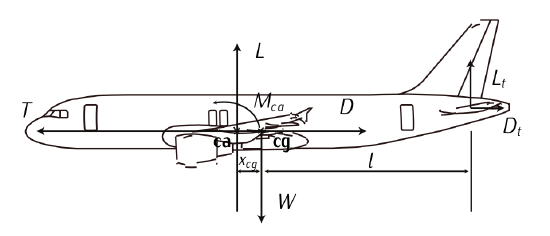
Figure 7.18: Longitudinal equilibrium.

Exercise \(\PageIndex{6}\) Performances

Consider an Airbus A-320 with the following characteristics:

• \(m = 64\) tonnes.
• \(S_w = 122.6\ m^2\)
• \(T_{\max, av, 0} = 130000\ N\) (maximum available thrust at sea level).
• \(C_D = 0.024 + 0.0375 C_L^2\).

The maximum available thrust can be considered to vary according to the following law:

\[T_{\max, av} (h) = T_{\max, av, 0} \dfrac{\rho}{\rho_0}.\nonumber\]

Consider \(ISA\) atmosphere and constant gravity \(g = 9.8\ m/s^2\).

1. The aircraft starts an uniform ascent maneuver (constant speed and flight path angle) at an altitude of 10.000 feet (\(3048\ m\)). At this flight level, the aerodynamic speed is \(150\ m/s\) and the vertical speed is \(12\ m/s\). Assuming a small angle of attack \(\gamma \ll 1\), calculate:
   (a) The ascent flight path angle, \(\gamma\).
   (b) The required thrust at these conditions.
   (c) Thust relation¹⁴ with respect to the maximum available thrust at that altitude.
2. Calculate the maximum angle of ascent (flight path angle) in uniform ascent at an altitude of 10000 feet. In these conditions, determine:
   (a) The aerodynamic speed and the vertical speed.
3. We want now to analyze the turn performances in the horizontal plane. Consider sea level conditions, maximum aerodynamic efficiency, and structural limitations characterized by a maximum load factor of \(n_{\max} = 2.5\). In these conditions, calculate:
   (a) The required bank angle.
   (b) Speed an radius of turn.
   (c) The required thrust.
   (d) Can the aircraft perform the complete turn?

Answer

Besides the data given in the statement, the following data have been used:

• \(g = 9.81\ m/s^2\).
• \(R = 287\ J/(kgK)\).
• \(\alpha_T = 6.5 \cdot 10^{-3}\ K/m\).
• \(\rho_0 = 1.225\ kg/m^3\).
• \(T_0 = 288.15\ K\).
• \(ISA: \rho = \rho_0 (1 - \dfrac{\alpha_T h}{T_0})^{\tfrac{gR}{\alpha_T} - 1}\).

1. Uniform-ascent under the following flight conditions:
   \(\bullet\) \(h = 3048\ m\). Using \(ISA \to \rho = 0.904\ kg/m^3\).
   \(\bullet\) \(V = 150\ m/s\).
   \(\bullet\) \(\dot{h}_e = 12\ m/s\).
   The system that governs the motion of the aircraft is:
   \[T = D + mg \sin \gamma;\label{eq7.3.114}\]
   \[L = mg \cos \gamma;\label{eq7.3.115}\]
   \[\dot{x}_e = V \cos \gamma;\label{eq7.3.116}\]
   \[\dot{h}_e = V \sin \gamma.\label{eq7.3.117}\]
   Assuming that \(\gamma \ll 1\), and thus that \(\cos \gamma \sim 1\) and \(\sin \gamma \sim \gamma\), System (\(\ref{eq7.3.114}\), \(\ref{eq7.3.115}\), \(\ref{eq7.3.116}\), \(\ref{eq7.3.117}\)) becomes:
   \[T = D + mg \gamma;\label{eq7.3.118}\]
   \[L = mg;\label{eq7.3.119}\]
   \[\dot{x}_e = V;\label{eq7.3.120}\]
   \[\dot{h}_e = V_{\gamma}. \label{eq7.3.121}\]
   (a) From Equation \(\ref{eq7.3.121}\), \(\gamma = \tfrac{\dot{h}_e}{V} = 0.08\ rad (4.58^{\circ})\).
   (b) From Equation \(\ref{eq7.3.118}\), \(T = D + mg\gamma\).
   \[D = C_D \dfrac{1}{2} \rho S_w V^2,\label{eq7.3.122}\]
   where \(C_D = 0.024 + 0.0375 C_L^2\), and \(\rho, S_w, V^2\) are known.
   \[C_L = \dfrac{L}{\tfrac{1}{2} \rho S_w V^2} = 0.5057.\label{eq7.3.123}\]
   where, according to Equation (\(\ref{eq7.3.119}\)), \(L = mg\). With Equation (\(\ref{eq7.3.123}\)) in Equation (\(\ref{eq7.3.122}\)), \(D = 41398\ N\).
   Finally:
   \[T = D + mg \gamma = 91886\ N.\nonumber\]
   (c) The maximum thrust at those conditions is 
   \[T_{\max, av} (h = 3048) = T_{\max, av, 0} \dfrac{\rho}{\rho_0} = 95510\ N.\nonumber\]
   The relation is \(\sqcap = \tfrac{T}{T_{\max, av}} = 0.962\).
2. Maximum angle of ascent.
   We consider again the set of equations (\(\ref{eq7.3.118}\), \(\ref{eq7.3.119}\), \(\ref{eq7.3.120}\), \(\ref{eq7.3.121}\)). Diving Equation (\(\ref{eq7.3.118}\)) by \(mg\), we have that:
   \[\gamma = \dfrac{T}{mg} - \dfrac{1}{E}.\]
   In order \(\gamma\) to be maximum:
   \(\bullet\) \(T = T_{\max, av} = 95510\ N\).
   \(\bullet\) \(E = E_{\max}\).
   Let us now proceed deducing the maximum aerodynamic efficiency:
   The aerodynamic efficiency is defined as:
   \[E = \dfrac{L}{D} = \dfrac{C_L}{C_D}.\label{eq7.3.125}\]
   Substituting the parabolic polar curve given in the statement in Equation (\(\ref{eq7.3.125}\)), we obtain:
   \[E = \dfrac{C_L}{C_{D_0} + C_{D_i} C_L^2}.\label{eq7.3.126}\]
   In order to seek the values corresponding to the maximum aerodynamic efficiency, one must derivate and make it equal to zero, that is:
   \[\dfrac{dE}{dC_L} = 0 = \dfrac{C_{D_0} - C_{D_i} C_L^2}{(C_{D_0} - C_{D_i} C_L^2)^2} \to (C_L)_{E_{\max}} = C_{L_{opt}} = \sqrt{\dfrac{C_{D_0}}{C_{D_i}}}.\label{eq7.3.127}\]
   Substituting the value of \(C_{L_{opt}}\) into Equation (\(\ref{eq7.3.126}\)) and simplifying we obtain that:
   \[E_{\max} = \dfrac{1}{2\sqrt{C_{D_0} C_{D_i}}}.\nonumber\]
   Substituting: \(C_{L_{opt}} = 0.8, E_{\max} = 16.66\), and \(\gamma_{\max} = 5.27^{\circ}\).
   The aerodynamic velocity will be given by:
   \[V = \sqrt{\dfrac{m \cdot g}{\tfrac{1}{2} \rho S_w C_{L_{opt}}}} = 119\ m/s.\nonumber\]
   From Equation (\(\ref{eq7.3.117}\)), \(\dot{h}_e = V \cdot \gamma = 10.95\ m/s\).
3. We want to perform a horizontal turn at an altitude of \(h = 0\) with a load factor \(n = 2.5 = n_{\max}\), and with the velocity corresponding to the maximum aerodynamic efficiency in horizontal, steady, straight flight.
   The equations governing the dynamics of the airplane in an horizontal turn are:
   \[T = D;\label{eq7.3.128}\]
   \[mV \dot{\chi} = L \sin \mu;\label{eq7.3.129}\]
   \[L \cos \mu = mg.\label{eq7.3.130}\]
   In a uniform (stationary) circular movement, it is well known that the tangential velocity is equal to the angular velocity \(\dot{\chi}\) multiplied by the radius of turn \(R\):
   \[V = \dot{\chi} R.\]
   Therefore, System (\(\ref{eq7.3.128}\), \(\ref{eq7.3.129}\), \(\ref{eq7.3.130}\)) can be rewritten as:
   \[T = D;\label{eq7.3.132}\]
   \[n \sin \mu = \dfrac{V^2}{gR};\label{eq7.3.133}\]
   \[n = \dfrac{1}{\cos \mu};\label{eq7.3.134}\]
   where \(n = \tfrac{L}{mg}\) is the load factor.
   (a). The required bank angle:
   Therefore, looking at Equation (\(\ref{eq7.3.134}\)), it is straightforward to determine that the bank angle of turn is \(\mu = 66.4^{\circ}\).
   (b). Velocity and radius of turn.
   First, we need to calculate the velocity corresponding to the maximum efficiency. As we have calculated before in Equation (\(\ref{eq7.3.127}\)), the coefficient of lift that generates maximum efficiency is the so-called optimal coefficient of lift, that is, \(C_{L_{opt}} = \sqrt{\tfrac{C_{D_0}}{C_{D_i}}} = 0.8\). The velocity yields then:
   \[V = \sqrt{\dfrac{L}{\tfrac{1}{2} \rho_0 S_w C_{L_{opt}}}} = 161.57\ m/s.\nonumber\]
   Entering in Equation (\(\ref{eq7.3.133}\)) with \(\mu = 66.4\) [deg] and \(V = 161.57\ m/s\); \(R = 1167\ m\).
   (c) The required thrust.
   Equation (\(\ref{eq7.3.132}\)) can be expressed as:
   \[T = \dfrac{1}{2} \rho_0 S_w V^2 C_{D_0} + \dfrac{L^2}{\tfrac{1}{2} \rho_0 V^2 S_w} C_{D_i}.\nonumber\]
   Since all values are known: \(T = 94093\ N\)
   (d). Since \(T \le T_{\max, av} (h = 0)\), the aircraft can perform the turn.

---

9. All this variables can be considered constant during take off.

10. Notice that given an altitude and a thrust setting, the aircraft can theoretically fly at two different velocities meanwhile those velocities lay between the minimum velocity (stall) and a maximum velocity (typically near the divergence velocity).

11. \(g\) represents the force due to gravity.

12. Notice that we can convert mass in weight by simply multiplying by the force due to gravity.

13. Notice that given an altitude and a thrust setting, the aircraft can theoretically fly at two different velocities meanwhile those velocities lay between the minimum velocity (stall) and a maximum velocity (typically near the divergence velocity).

14. It refers to a value between 0 & 1 associated to the throttle level position.