5.1: Plant Production in Controlled Environments

Timothy J. Shelford

Department of Biological and Environmental Engineering

Cornell University

Ithaca, NY, USA

A. J. Both

Department of Environmental Sciences

Rutgers University

New Brunswick, NJ, USA

Key Terms

Psychrometric chart	Shading	Ventilation
Heating	Mechanical cooling	Installation cost
Lighting	Evaporative cooling	Operating cost

Variables

• ρ_i = density of the greenhouse air
• A_c = area of the greenhouse surface (walls and roof)
• c_ρi = specific heat of air in the greenhouse
• h_fg = latent heat of vaporization of water at t_i
• N = infiltration rate
• q_ccr = heat loss by conduction, convection, and radiation
• q_i = heat loss by infiltration
• t_i = inside air temperature of the greenhouse
• t_o = temperature of the ambient air (outside air)
• T_d = dew point air temperature
• T_db = dry-bulb air temperature
• T_wb = wet-bulb air temperature
• U = overall heat transfer coefficient
• V = volume of the greenhouse
• W_i = humidity ratio of the greenhouse air
• W_o = humidity ratio of the outside air

Introduction

Controlled environment crop production involves the use of structures and technologies to minimize or eliminate the potentially negative impact of the weather on plant growth and development. Common structures include greenhouses (which can be equipped with a range of technologies depending on economics, crops grown and grower preferences), and indoor growing facilities (e.g., growth chambers, plant factories, shipping containers, and vertical farms in high-rise buildings). While each type of growing facility has unique challenges, many of the processes, principles, and technology solutions are similar. This chapter describes approaches to environmental control in plant production facilities with a focus on technologies used for crop production and light control.

Outcomes

After reading this chapter, you should be able to:

• • List and explain the critical environmental control challenges for plant production in controlled environments
• • Perform design calculations for systems used for plant production in controlled environments
• • Calculate the installation and operating cost estimates of lighting systems for plant production in controlled environments

Concepts

Greenhouses were developed to extend the growing season in colder climates and to allow the production of perennial plants that would not naturally survive cold winter months. In providing an optimal environment for a crop, whether in a greenhouse or indoor growing facility, the air temperature is a critical factor that impacts plant growth and development. An equally important and related factor is the moisture content of the air (expressed as relative humidity). Plant growth depends on transpiration, a process by which water and nutrients from the roots are drawn up through the plant, culminating in evaporation of the water through the stomates located in the leaves. (Stomates are small openings that allow for gas exchange. They are actively controlled by the plant.) The transpiration of water through the stomates also results in cooling. Under high relative humidity conditions, the plant is unable to transpire effectively, resulting in reduced growth and, in some cases, physiological damage. Growers seek to create ideal growing environments in greenhouses and other indoor growing facilities by controlling heating, venting, and cooling (Both et al., 2015).

Psychrometric Chart

Knowledge of the relationship between temperature and relative humidity is critical in the design of heating, cooling, and venting systems to maintain the desired environmental conditions inside plant production facilities. The psychrometric chart (Figure 5.1.1) is a convenient tool to help determine the properties of moist air. With values of only two parameters (e.g., dry-bulb temperature and relative humidity, or dry-bulb and wet-bulb temperatures), other air properties can be read from the chart (some interpolation may be necessary). The fundamental physical properties of air used in the psychrometric chart are described below.

Figure \(\PageIndex{1}\): Example psychrometric chart used to determine the physical properties of air. Curved green lines: constant relative humidity; steep blue straight lines: constant specific volume; less steep red straight lines: constant enthalpy.

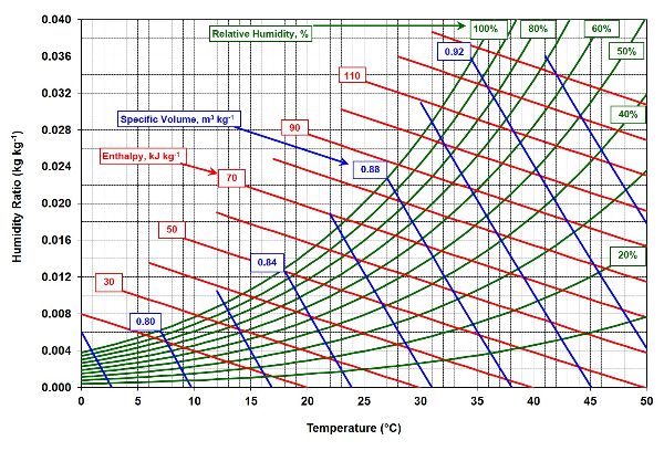
• • Dry-bulb temperature (T_db, °C) is air temperature measured with a regular thermometer. In a psychrometric chart (Figure 5.1.1), the dry-bulb temperature is read from the horizontal axis.
• • Wet-bulb temperature (T_wb, °C) is air temperature measured when air is cooled to saturation (i.e., 100% relative humidity) by evaporating water into it. The energy (latent heat) required to evaporate the water comes from the air itself. The wet-bulb temperature can be measured by keeping the sensing tip of a thermometer moist (e.g., by surrounding it with a wick connected to a water reservoir) while the thermometer is moved through the air rapidly, or by blowing air through the moist (and stationary) sensing tip. In a psychrometric chart (Figure 5.1.1), the wet-bulb temperature is read from the horizontal axis by following the line of constant enthalpy from the initial condition (e.g., the intersection of dry-bulb temperature and relative humidity combination) to the saturation line (100% relative humidity).
•  
• • Dewpoint temperature (T_d, °C) is the air temperature at which condensation occurs when moist air is cooled. In a psychrometric chart (Figure 5.1.1), the dewpoint temperature is read from the horizontal axis after a horizontal line of constant humidity ratio is extended from the initial condition (e.g., the intersection of dry-bulb temperature and relative humidity combination) to the saturation line (100% relative humidity).
• • Relative humidity (RH, %) is the level of air saturation (with water vapor). In a psychrometric chart (Figure 5.1.1), curved lines are of constant relative humidity.
• • The humidity ratio (kg kg⁻¹) is the mass of water vapor evaporated into a unit mass of dry air. In a psychrometric chart (Figure 5.1.1), the humidity ratio is read from the vertical axis.
• • Enthalpy (kJ kg⁻¹) is the energy content of a unit mass of dry air, including any contained water vapor. The psychrometric chart (Figure 5.1.1) typically presents lines of constant enthalpy.
• • Specific volume (m³ kg⁻¹) is the volume of a unit mass of dry air; it is the inverse of the air density. The psychrometric chart (Figure 5.1.1) presents lines of constant specific volume.

Heating

A major expense of operating a greenhouse year-round in cold climates is the cost of heating. It is, therefore, important to understand the major modes of heat loss when designing or operating a greenhouse. Heat loss occurs from the structure directly through conduction, convection, and radiation. Depending on location, when estimating heat losses, it may be necessary to include heat loss around the outside perimeter, as well as the impact of high outside wind speeds and/or large temperature differences between the inside and outside of the greenhouse (Aldrich and Bartok, 1994).

Estimating Heat Needs

Estimating the heat losses due to conduction, convection, radiation, and infiltration, requires both the inside and outside air temperatures. The inside air temperature is usually based on the nighttime set point required by the crop. In the absence of specific crop requirements, typically 16°C can be used as a minimum. If the greenhouse is to be used year-round, typically the 99% winter design dry-bulb temperature is used for the outside temperature. The 99% winter design dry-bulb temperature is the outdoor temperature that is only exceeded 1% of the time (based on 30 years of data for the months December, January, and February collected at or near the greenhouse location). The term “exceeded” in the previous sentence means “colder than.” Such values for many locations throughout the world are published by ASHRAE (2013).

Calculating the exchange of heat (by conduction, convection, and radiation) is a complex process that usually involves making many simplifying assumptions. Solutions often require iterative calculations that are tedious without the help of computing tools. Computing software such as EnergyPlus™ (Crawley, 2001) and Virtual Grower (USDA-ARS, 2019) are available for heat loss calculations. However, even software packages developed for heat loss calculations may not necessarily provide accurate results.

Other methods that greatly simplify performing heat loss calculations using heat transfer coefficients are available. Heat transfer coefficients combine the effects of conduction, convection, and radiation in a single coefficient. Since these processes depend on many factors other than the temperature differential, their accuracy is not high, especially when conditions are extreme, or outside of typical operating ranges. However, for quick estimates that are not computationally intensive, coefficient-based calculations may be useful to a designer or operator. Equation 5.1.1 provides a means to solve for the conductive, convective, and radiative heat losses:

\[ q_{ccr} = UA_{c}(t_{i} - t_{o}) \]

where q_ccr = heat loss by conduction, convection, and radiation (W)

U = overall heat transfer coefficient (W m⁻² °C⁻¹)

A_c = area of the greenhouse surface (walls and roof) (m²)

t_o = ambient (outside) air temperature (°C); the 99% design temperature is commonly used for this parameter (see text)

The overall heat transfer coefficients for typical greenhouse materials are listed in Table 5.1.1.

Equation 5.1.2 is for solving the heat loss due to infiltration:

\[ q_{i} = \rho_{i} NV[c_{pi(t_{i}-t_{o})}+h_{fg}(W_{i}-W_{o})] \]

where q_i = heat loss by infiltration (W)

ρ_i = density of the greenhouse air (kg m⁻³)

N = infiltration rate (s⁻¹)

V = volume of the greenhouse (m³)

c_ρi = specific heat of the greenhouse air (J kg⁻¹ °C⁻¹)

t_i = greenhouse (inside) air temperature (°C)

t_o = outside air temperature (°C)

h_fg = latent heat of vaporization of water at t_i (J kg⁻¹)

W_i = humidity ratio of the greenhouse air (kg_water kg_air⁻¹)

W_o= humidity ratio of the outside air (kg_water kg_air⁻¹)

Table \(\PageIndex{1}\): Approximate overall heat transfer coefficients (U-values) for select greenhouse glazing methods and materials (ASAE Standards, 2003).

Greenhouse Covering	U Value (W m^−2 °C^−1)
Single glass, sealed	6.2
Single glass, low emissivity	5.4
Double glass, sealed	3.7
Single plastic	6.2
Single polycarbonate, corrugated	6.2–6.8
Single fiberglass, corrugated	5.7
Double polyethylene	4
Double polyethylene, IR inhibited	2.8
Rigid acrylic, double-wall	3.2
Rigid polycarbonate, double-wall^1	3.2–3.6
Rigid acrylic, w/polystyrene pellets^2	0.57
Double polyethylene over glass	2.8
Single glass and thermal curtain^3	4
Double polyethylene and thermal curtain^3	2.5

¹ Depending upon the spacing between walls.

² 32 mm rigid acrylic panels filled with polystyrene pellets.

³ Only when the curtain is closed and well-sealed.

Select heat transfer coefficients (U-values; Table 5.1.1) and infiltration rates (Table 5.1.2) with caution when performing heat loss calculations. Infiltration rates depend highly on the magnitude and direction of the wind, among other factors.

Cooling and Cooling Methods

During warmer periods of the year, the temperature inside the growing area of a plant production facility could be much higher than the outside temperature (as occurs inside a closed car on a sunny day). High temperatures inside greenhouses can depress plant growth and, in extreme cases, kill a crop. Cooling systems are essential for plant production facilities that are used year-round.

Table \(\PageIndex{2}\): Estimated infiltration rates for greenhouses by type and age of construction (ASAE Standards, 2003).

Type and Construction	Infiltration Rate (N)^1
New construction:	s^−1	h^−1
Double plastic film	2.13 × 10^−4–4.13 × 10^−4	0.75–1.5
Glass or fiberglass	1.43 × 10^−4–2.83 × 10^−4	0.50–1.0
Old construction:
Glass, good maintenance	2.83 × 10^−4–5.63 × 10^−4	1.0–2.0
Glass, poor maintenance	5.63 × 10^−4–11.13 × 10^−4	2.0–4.0

¹ Internal air volume exchanges per unit time (s⁻¹ or h⁻¹). High winds or direct exposure to wind will increase infiltration rates; conversely, low winds or protection from wind will reduce infiltration rates.

Mechanical Cooling (Air Conditioning)

Although air conditioning of greenhouses is technically feasible, the installation and operating costs can be very high, particularly during the summer months. The most economical time to use air conditioners in greenhouses is during the spring and autumn when the heat load is relatively low and the crop may benefit from CO₂ enrichment. Air conditioning is an alternative to using ventilation to manage humidity and control temperature. By definition, air conditioning is a thermodynamic process that removes heat and moisture from an interior space (e.g., the interior of a controlled environment plant production facility) to improve its conditions. It involves a mechanical refrigeration cycle that forces a refrigerant through a circular process of expansion and contraction, resulting in evaporation and condensation, resulting in the extraction of heat (and moisture) from the plant growing area.

Mechanical cooling may be necessary for indoor growing facilities. Typically, indoor growing facilities operate with minimal exchange rates with the outside air, and so air conditioning becomes one of the ways to remove the humidity generated by plants during transpiration. It is essential to insulate and construct the building properly to minimize solar heat gain in indoor facilities that may add to the heat load. Additionally, it is crucial to know the heat load from electric lamps providing the energy needed for photosynthesis to size the air conditioner adequately.

Evaporative Cooling

Sometimes during the warm summer months, regular ventilation and shading (e.g., whitewash or movable curtains) are not able to keep the greenhouse temperature at the desired set point, thus, additional cooling is needed. Growers typically use evaporative cooling as a simple and relatively inexpensive cooling method. The process of evaporation requires heat. This heat (energy) comes from the surrounding air, thereby causing the air temperature to drop. Simultaneously, the humidity of the air increases as the evaporated water becomes part of the surrounding air mass. The maximum amount of cooling possible with evaporative cooling systems depends on the initial properties of the outside air, i.e., the relative humidity (the drier the air, the more water it can absorb, and the lower the final air temperature will be) and air temperature (warmer air can carry more water vapor compared to colder air). Two different evaporative cooling systems used to manage greenhouse indoor air temperatures during periods when using outside air for ventilation is not sufficient to maintain the set point temperatures are the pad-and-fan system and the fog system.

Pad-and-Fan System

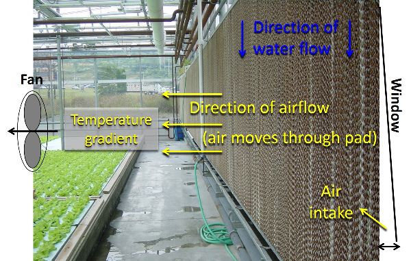
Pad-and-fan systems include an evaporative cooling pad installed as a segment of the greenhouse wall, typically on the wall opposite the exhaust fans. Correctly installed pads allow all incoming ventilation air to pass through it before entering the greenhouse environment (Figure 5.1.2). The pads are made from corrugated material (impregnated paper or plastic) glued together in a way that allows maximum contact with the air passing through the wet pad material. Water is introduced at the top of the pad and released through small holes along the entire length of the supply pipe. These holes are spaced uniformly along the whole length of the pad to provide even wetting. Excess water is collected at the bottom of the pad and returned to a sump tank for reuse. The sump tank is fitted with a float valve to manage make-up water that compensates for the portion of the recirculating water lost through evaporation and to dilute the salt concentration that may increase in the remaining water over time. It is common practice to continuously bleed off approximately 10% of the returning water to a designated drain to prevent excessive salt build-up (crystals) on the pad material that may reduce pad efficiency. During summer operation, it is common to “run the pads dry,” i.e., to stop the flow of water while keeping the ventilation fans running at night to prevent algae build-up that can also reduce pad efficiency. The cooled (and humidified) air exits the pad and moves through the greenhouse picking up heat from the greenhouse interior. In general, pad-and-fan systems used in greenhouses experience a temperature gradient between the inlet (pad) and the outlet (exhaust fan). In properly designed systems, this temperature gradient is kept low (up to 4°–6°C is possible) to provide a uniform environment for all the plants.

Figure \(\PageIndex{2}\): Main design features of a pad-and-fan evaporative cooling system. Water is supplied by a pump from a reservoir and is recirculated. (Photo by A. J. Both)

The required evaporative pad area depends on the pad thickness and can be calculated by:

\[ A_{pad} = \frac{\text{total greenhouse ventilation fan capacity}}{\text{recommended air velocity through pad}} \]

For example, for 10 cm thick pads, the fan capacity (in m³ s⁻¹) should be divided by the recommended air velocity through the pad, 1.3 m s⁻¹ (ASAE Standards, 2003). For 15 cm thick pads, the fan capacity should be divided by the recommended air velocity through the pad, 1.8 m s⁻¹. The recommended minimum pump capacity is 26 and 42 L s⁻¹ per linear meter of the pad, and the minimum sump tank capacity is 33 and 41 L per m² of pad area for the 10 and 15 cm pads, respectively. For evaporative cooling pads, the estimated maximum water usage can be as high as 17–20 L h⁻¹ per m² of pad area.

High-Pressure Fog System

The other evaporative cooling system commonly used is the fog system. This system is typically used in greenhouses with natural ventilation systems because natural ventilation does not have the force to overcome the additional resistance to airflow resulting from an evaporative cooling pad. The nozzles of a fog system are typically installed throughout the greenhouse to provide a more uniform cooling pattern compared to the pad-and-fan system. The recommended spacing is approximately one nozzle for every 5–10 m² of growing area. The water pressure used in greenhouse fog systems is relatively high (≥3,450 kPa) and enough to produce very fine droplets that evaporate before reaching plant surfaces. The water usage per nozzle is small, approximately 3.8–4.5 L h⁻¹. Water for fogging systems should be free of any impurities to prevent clogging of the nozzle openings. Therefore, fog systems require water treatment (filtration and purification) and a high-pressure pump. Thus, fog systems can be more expensive to install compared to pad-and-fan systems, but the resulting cooling is more uniform.

Ventilation

To maintain optimum growing conditions, warm and humid indoor air needs to be replaced with cooler and drier outside air. Plant production facilities use either mechanical or natural ventilation to accomplish this. Mechanical ventilation requires inlet openings, exhaust fans, and electric power to operate the fans. When appropriately designed, mechanical ventilation can provide adequate cooling and dehumidification under a wide range of weather conditions throughout many locations with temperate climates. The typical design specification for maximum mechanical ventilation capacity is 0.05 or 0.06 m³ s⁻¹ per m² of floor area for greenhouses with or without a shade curtain, respectively. When deliberate obstructions to the air intake are present (such as insect exclusion screens and an evaporative cooling pad), the inlet area should be carefully sized to overcome the increased resistance to airflow that would result in a reduction in the total air exchange rate relative to fully opened and unobstructed inlets. In that case, ventilation fans should be able to overcome the additional airflow resistance created by the screen or evaporative cooling pad. Multiple and staged fans can provide different ventilation rates based on environmental conditions. Variable-speed fan motors allow for more precise control of the ventilation rate and can reduce overall electricity consumption.

Natural ventilation works on two physical phenomena: thermal buoyancy (warm air is less dense and rises), and the wind effect (wind blowing outside a structure creates small pressure differences between the windward and leeward sides of the structure causing air to move towards the leeward side). All that is needed are carefully placed inlet and outlet openings, vent window motors, and electricity to operate the motors. In some naturally ventilated greenhouses, the vent window positions are managed manually (e.g., in a low-tech plastic tunnel production system), eliminating the need for motors and electricity, but this increases the amount of labor, especially where frequent adjustments are necessary. Electrically operated natural ventilation systems use much less power than mechanical (fan) ventilation systems. When using a natural ventilation system, additional cooling can be provided by a fog system, for example, provided the humidity of the air is not too high. Unfortunately, natural ventilation does not work very well on warm days when the wind velocity is low (less than 1 m s⁻¹) or when the facility uses a shade system that obstructs airflow. When using natural or forced ventilation alone, the indoor temperature cannot be lowered below the outdoor temperature without additional cooling capabilities (typically evaporative cooling).

For most freestanding greenhouses, mechanical ventilation systems usually move the air along the length of the greenhouse (i.e., the exhaust fans and inlet openings are installed in opposite end walls). To avoid excessive airspeed within the greenhouse, the inlet to fan distances are generally limited to 70 to 80 m, provided local climates are not too hot. Natural ventilation systems for freestanding greenhouses usually provide cross ventilation using sidewall windows and roof vents.

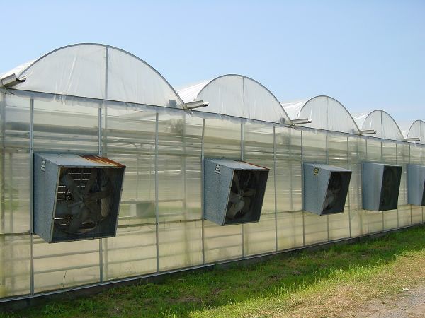
In gutter-connected greenhouses (Figure 5.1.3), mechanical ventilation system inlets and outlets can be installed in the side or end walls, while natural ventilation systems usually consist of only roof vents. Sidewall vents have limited influence on the ventilation of interior sections in larger greenhouses. The ultimate natural ventilation system is the open-roof greenhouse design that allows for the indoor temperature to seldom exceed the outdoor temperature. This kind of effect is not attainable with mechanically ventilated greenhouses due to the substantial amounts of air that such systems would have to move through the greenhouse to accomplish the same results.

Figure \(\PageIndex{3}\): Gutter-connected greenhouses with mechanical ventilation. (Photo by A. J. Both)

Whatever the ventilation system used, uniform air distribution inside the greenhouse is essential because uniformity in crop production is only possible when all plants experience the same environmental conditions. Therefore, the use of horizontal airflow fans is common to ensure proper air mixing. The recommended horizontal airflow fan capacity is approximately 0.015 m³ s⁻¹ per m² of the growing area.

Lighting and Shading

Since light is the driving force for photosynthesis and plant growth, managing the light environment of a growing facility is of prime importance. For many crops, plant growth is proportional to the amount of light the crop receives over the entire growing period. Both the instantaneous light intensity and the daily light integral are important parameters to growers. Plant scientists define light in the 400–700 nm waveband as photosynthetically active radiation (PAR). PAR represents the (instantaneous) light intensity and has the units μmol m⁻² s⁻¹ (ASABE Standards, 2017). When referring to the amount of light a crop receives over some time, such as an hour or a day, the sum of the instantaneous PAR intensities is calculated, and the resulting values are often called light integrals. Usually, growers measure light integrals over an entire day (sunrise to sunrise), resulting in the daily light integral (DLI), with the unit mol m⁻² d⁻¹. Instantaneous measures of PAR may be used to trigger control actions such as turning supplemental lighting on or off. Some growers deploy movable shade curtains to manage the light intensity. Daily light integrals (DLIs) can be used by growers to ensure a consistent level of crop growth by maintaining a consistent integral from day to day (whether from natural light, supplemental lighting, or a mix), or to track the accumulated radiation input that serves as the energy source for photosynthesis. The total DLI received by a plant canopy is the sum of the amount of sunlight received plus any contribution from the supplemental lighting system (for greenhouse production). Equation 5.1.4 determines the instantaneous PAR intensity (μmol m⁻² s⁻¹) necessary to meet a DLI target (mol m⁻² d⁻¹) over a specific number of hours:

\[ \text{intensity}(\frac{\mu mol}{m^{2}s}) = \frac{DLI}{\text{h per day}} \times \frac{1\ h}{3,600\ s} \times \frac{1\times10^{6} \mu mol}{1\ mol} \]

For example, using Equation 5.1.4, an intensity of 197 μmol m⁻² s⁻¹ is needed to deliver a target DLI of 17 mol m⁻² d⁻¹ over 24 h (one day).

Plant Sensitivity to Light

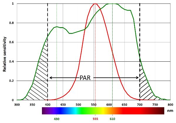
Human eyes have a different sensitivity to (natural) light (or radiation) compared to how plants respond to light (Figure 5.1.4). Human eyes are most sensitive to green wavelengths (peak at 555 nm), while most plants exhibit peak sensitivities in the blue (peaking at 430 nm) and orange-red part (peaking at 610 nm) of the visible light spectrum. This difference in sensitivity means the human eye is not a very useful “sensor” in terms of assessing whether a particular light environment is suitable for plant growth and development. While PAR is light across the 400–700 nm waveband, as shown in Figure 5.1.4, plants are also sensitive to UV (280–400 nm) and far-red (700–800 nm) radiation. Therefore, it is best to use specially designed sensors (PAR sensors and spectroradiometers) to evaluate the light characteristics in environments used for plant production.

Natural and Electric Lighting

Natural light from the sun is an essential aspect of greenhouse production, both in terms of plant growth and development, but also in terms of energy balance (greenhouse heating and cooling). In indoor growing facilities, light is solely provided by electric lighting, though the amount of natural light striking the external surface of the building containing an indoor growing facility can also substantially affect the energy balance of the facility.

Figure \(\PageIndex{4}\): Differences in relative light sensitivity comparing the human eye (red line) to an average plant (green line). PAR = photosynthetically active radiation (400–700 nm). Horizontal axis: wavelength in nanometers. Sources: Commission Internationale de l’Eclairage (1931) and Sager et al. (1988).

Direct and Diffuse Sunlight

The earth’s atmosphere contains many particles (gas molecules, water vapor, and particulate matter) that can change the direction of the light from the sun. On a clear day, there are fewer particles in the atmosphere, and sunlight travels unimpeded before reaching the ground. This type of sunlight is called direct light or direct radiation. On cloudy days, the atmosphere contains more particles (mainly water vapor), and the interaction of sunlight with all those particles causes directional changes that are mostly random. As a result, on cloudy days, sunlight comes from many directions. This type of sunlight is called diffuse light or diffuse radiation. These frequent light-particle interactions will also result in a reduction in light intensity compared to direct radiation.

Depending on the make-up of the atmosphere (cloudiness), sunlight will reach the surface as direct radiation, diffuse radiation, or a combination of the two. Direct radiation does not reach the lower canopy layers shaded by plant tissues (mostly leaves); however, because diffuse radiation is omnidirectional, it can penetrate deeper into a plant canopy (particularly in a multi-layered, taller canopy). Therefore, though the amount of diffuse radiation may appear small, it can boost plant production because it reaches more of the plant surfaces involved in photosynthesis. Some greenhouse glazing materials (e.g., polyethylene film) diffuse incoming solar radiation more than others (Table 5.1.3), and while the overall light intensity is often lower in greenhouses covered with a diffusing glazing material, crop growth and development is not necessarily reduced proportionally because more of the canopy surfaces are receiving adequate light for photosynthesis.

The amounts of diffuse radiation are measured with a light sensor placed behind a disc that casts a precise shadow over the sensor, so it blocks all direct radiation. The amount of direct radiation is determined by using a second sensor that measures total (direct plus diffuse) radiation (direct radiation = total radiation – diffuse radiation).

Table \(\PageIndex{3}\): Characteristics of glazing materials.

Glazing Material	Direct PAR Transmittance (%)	Infrared (heat) Transmittance[a] (%)	Ultraviolet Transmittance[b] (%)	Life Expectancy (years)
Glass	90	0	60–70	30
Acrylic[c]	89	0	44	10–15
Polycarbonate3	80	0	18	10–15
Polyethylene[d]	90	45	80	3–4
PE, IR & AC[d][e]	90	30	80	3–4

[a] for wavelengths above 3,000 nm

[b] for wavelengths between 300 and 400 nm

[c] twin wall

[d] single layer

[e] polyethylene film with an infrared barrier and an anti-condensate surface treatment

As sunlight reaches the external surfaces of the greenhouse structure, the light can be reflected, absorbed, or transmitted. Often these processes coincide. The quantities of reflected, absorbed, or transmitted light depend on the (glazing) materials involved, the time of day, the time of year, and whether the grower uses any control strategies (e.g., whitewash or shade curtains). Also, overhead equipment can block light and reduce the total amount of sunlight that reaches the plant canopy. It is not uncommon, even in modern greenhouses, for the plants to receive around 50–60% on average of the amount of sunlight available outside the greenhouse structure. Since every percent of additional light received by the plant canopy counts, it is essential to design greenhouses carefully with optimum light transmission in mind.

Effect of Greenhouse Orientation

Another consideration, particularly at higher latitudes, is the orientation of the greenhouse. At latitudes above 40 degrees, orienting the gutters of a greenhouse along an east-west direction can help capture the most amount of light during the winter months when the sun is low in the sky and the total amount of sunlight is also low. However, using such an orientation, shadow bands created by structural components and overhead equipment tend to move more slowly. This can be a particularly challenging issue when the crop is grown in the greenhouse for only a short amount of time (e.g., for leafy greens). In that case, it is preferable to orient the greenhouse north-south. Aside from any shadows, the intensity of sunlight is considered uniform throughout the growing area.

Shading

During bright sunny days, there is the risk of greenhouse crops being exposed to too much light, thus requiring the use of shade curtains to help reduce plant stress from high light intensities. On variably cloudy days, the light conditions inside a greenhouse can fluctuate rapidly from low light to high light conditions. Such swings in light conditions can negatively impact plant growth and development, so growers may have to deploy both the supplemental lighting system and the shade curtains to provide more stable growing conditions. Managing the supplemental lighting system often involves controlling the shade curtains.

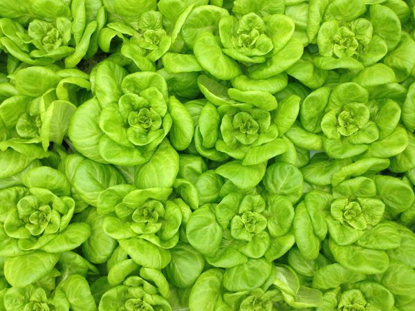
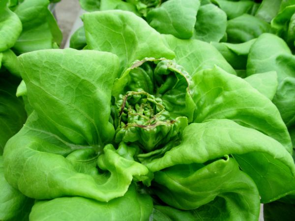
Proper shading is essential for some crops. For example, lettuce grown in a greenhouse is subject to tipburn (Figure 5.1.5) if light, temperature, and humidity conditions are not kept within specific ranges.

One strategy is to apply a whitewash treatment to the greenhouse during peak solar radiation months and to wash it off at the end of the natural growing season when light conditions diminish. Drawbacks include increased labor costs and additional requirements for supplemental lighting. Movable shade curtains are another effective strategy for managing tipburn, if properly designed and used. Deploying shade curtains too late during the day can cause tipburn in lettuce (too much light increases the growth rate beyond the point where the transport of calcium can keep up), and deploying them too early can result in extra hours of supplemental lighting. Movable shade curtains, depending on the design, can also reduce heat loss during the night, but this dual use is often a compromise between optimum shading capabilities and maximum energy retention. A more comprehensive solution is two different curtains, each optimized for its purpose, but such a dual curtain system doubles the installation cost.

Tipburn is a physiological disorder caused by calcium deficiency in leaf tips. It renders the product unsalable.

Figure \(\PageIndex{5}\): Example of lettuce plants without (top, photo by A. J. Both) and with tipburn (bottom, photo courtesy of the Cornell University Controlled Environment Agriculture Program).

Common Types of Artificial Lighting

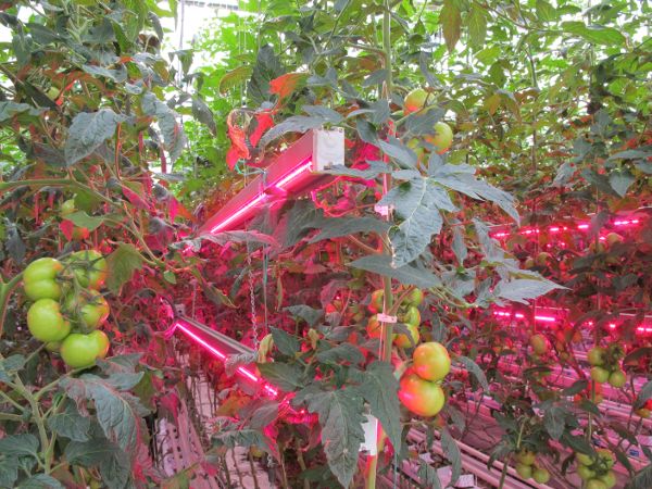
The two most common types of greenhouse lighting are gas discharge and light-emitting diode (LED) lamps (Figure 5.1.6). Gas discharge lamps, such as fluorescent (FL), metal halide (MH), and high-pressure sodium (HPS) lamps, produce light by passing a current through an ionized gas. The spectrum of light produced is a function of the gas used and the composition of the electrodes. MH lamps provide a more white-colored light, while HPS light is more yellowish orange (similar to traditional streetlamp light).

LED lamps use semiconductors that release energy in the form of photons when sufficient current is passed through them. The wavelength of light emitted is determined by the bandgap of the semiconductor and any phosphors used to convert the monochromatic LED light. Unlike gas discharge lamps, LEDs without phosphors produce light within a relatively narrow waveband. To get a broad-spectrum output, such as white light, manufacturers often use high-efficiency blue LEDs and convert the output to white light using yellow phosphors. Some plants benefit from small amounts of UV radiation (280–400 nm), but people working in these environments should wear special eye and skin protection to minimize the harmful effects presented by UV radiation.

Figure \(\PageIndex{6}\): High-pressure sodium fixtures mounted over a rose crop (top) and LED fixtures with a magenta color mounted within a tomato crop (bottom) (photos by A. J. Both).

Lighting Efficacy

At the time of this writing (early 2020), the most energy-efficient lamps available for supplemental lighting are LED-based fixtures (Mitchell et al., 2012; Wallace and Both, 2016). However, not all LED fixtures are designed for plant growth applications. When comparing the efficiency of lights, the wall-plug energy use of the fixture must be considered. Some LED fixtures rely on active cooling using ventilation fans (in some cases water cooling) to prevent overheating that can shorten their lifespans. Active cooling installation requires additional energy, which must be considered, in addition to other losses, such as from transformers and drivers. Ideally, manufacturers publish an efficacy measurement, i.e., light output divided by energy input, or μmol s⁻¹ of PAR (light) output per W (electricity) input (μmol J⁻¹) for their fixtures (Both et al., 2017). Efficacies for lamps used in plant growth applications are shown in Table 5.1.4. Fixture efficacies continue to increase with several LED fixtures now approaching 3 μmol J⁻¹. Higher efficacy fixtures use less electrical energy to produce the same amount of light.

A Note on Lighting Units

In the horticulture industry, it is still common to use light units of lux, lumens, or foot-candles. However, this is not particularly useful since lux, lumens, and foot candles are based on the sensitivity of the human eye, which is most sensitive to the green part of the visible light spectrum (Figure 5.1.4). Ideally, the total light output of supplemental lighting devices should be reported in integrated PAR units (μmol s⁻¹). Note that this unit is not the same as the unit used for instantaneous PAR intensity (μmol m⁻² s⁻¹). Users should be aware of this when purchasing lighting fixtures and make sure that the proper instruments were used to assess the light output.

Table \(\PageIndex{4}\): Selected fixture efficacies for several different lamp types used for horticultural applications (CMH = ceramic metal halide, HPS = high-pressure sodium, LED = light emitting diode).

Lamp Type	Power Consumption (W)	Efficacy (μmol J^−1)
Incandescent (Edison bulb)	102.4	0.32
Compact fluorescent (large bulb)	61.4	0.89
CMH (mogul base)	339	1.58
HPS (mogul base)	700	1.56
HPS (double ended)	1077	1.59
LED (bar, passively cooled)	214	2.39

Advantages and Disadvantages of Lighting Systems

HPS Lighting System

HPS lamps have long been the preferred lamp type for supplemental lighting applications (Both et al., 1997).

Advantages

• • Both lamps and fixtures (including the ballasts and reflectors) are relatively inexpensive and easy to maintain (e.g., bulb replacement and reflector cleaning).
• • Before LEDs became available, HPS lamps had the highest conversion efficiency (efficacy), and they produced a sufficiently broad spectrum that was acceptable for a wide range of plant species. The recent introduction of double-ended HPS lamps somewhat increased their efficacy.

Disadvantages

• • A major drawback of HPS lamps is the production of a substantial amount of radiant energy, necessitating adequate distance between the lights and the plant surfaces exposed to this radiation.
• • They require a warm-up cycle before they reach maximum output, and once turned off, need a cool-down period before using again.
• • As with all lamps, the light output of HPS lamps depreciates over time, requiring bulb replacements every 10,000–15,000 hrs.

Since HPS lamps have been in use for several decades, researchers and growers have learned how best to produce their crops with this light source. For example, while the radiant heat production can be considered a drawback, it can also be used as a management tool to help maintain a desirable canopy temperature, and this radiant heat can help reduce the amount of heat energy (provided by the heating system) needed to keep the set point temperature.

LED Lighting Systems

LED lamps (often consisting of arrays of multiple individual LEDs) are a relatively new technology for horticultural applications, and their performance capabilities are still evolving (Mitchell et al., 2015).

Advantages

• • The efficacy of carefully designed LED lamps has surpassed the efficacy of HPS lamps, and the heat they produce can be removed more easily by either natural or forced convection.
• • The resulting convective heat (warm air emanating from the lamp/fixture) is easier to handle in controlled environment facilities than the radiant heat produced by HPS lamps because air handling is a common process while blocking radiant heat is not.
• • LED lamps can be switched on and off rapidly and require a much shorter warm-up period than HPS lamps.
• • It is possible to modulate the light intensity produced by LED lamps, either by adjusting the supply voltage or by a process called pulse width modulation (PWM; rapid on/off cycling during adjustable time intervals). By combining (and controlling) LEDs with different color outputs in a single fixture, growers have much more control over the spectrum that these lamps produce, opening up new strategies for growing their crops. This benefit in particular will require (a lot of) additional research to be fully understood or realized.
• • LED lamps typically have a longer operating life (up to 50,000 h), but more testing is needed in plant production facilities to validate this estimate.

Disadvantages

• • LED lamps (fixtures) are more expensive compared to HPS fixtures with similar output characteristics.
• • LED lamps typically come as a packaged unit (including LEDs, housing, and electronic driver), making the replacement of failed components almost impossible.
• • Because plants are most sensitive to blue and red light in terms of photosynthesis, growers often use LED fixtures that produce a combination of red + blue = magenta light. The magenta light (Figure 5.1.6) makes it much more challenging to observe the actual color of plant tissue (which is essential for the observation of potential abnormalities resulting from pest and/or disease issues), and can make working in an environment with that spectrum more challenging (it has been reported to make some people uncomfortable).
• • Some LED lamps have (unperceivable) flicker rates that can have health effects on humans with specific sensitivities (e.g., people with epilepsy).

Applications

Heating Systems in Greenhouses

Greenhouses can be heated using a variety of methods and equipment to manage heat losses during the cold season. Typically, fuel is combusted to heat either air or water (steam in older greenhouses) which is circulated through the greenhouse environment. Some greenhouses use infrared heating systems that radiate heat energy to exposed surfaces of the plant canopy. The use of electric (resistance) heating is minimal because of the high operating cost. However, as the costs of fossil fuels rise, electric heating could become competitive even for extensive greenhouse operations in various locations.

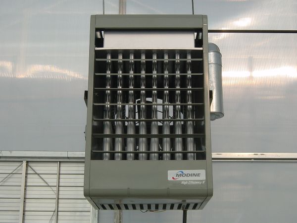
Unit Heaters and Furnaces

Typical air heating systems include unit heaters and furnaces (Figure 5.1.7). Typically, the heat generated by the combustion process is transferred to the greenhouse air through a heat exchanger, or the air from the greenhouse used as the oxygen source for the combustion process and then released into the greenhouse. Using heat exchangers allows for the combustion air to remain separate from the greenhouse environment (separated combustion), thus minimizing the risk of releasing small amounts of potentially harmful gasses (e.g., ethylene, carbon monoxide) into the greenhouse environment. Also, it directly increases the air temperature without introducing additional moisture.

Using greenhouse air as a source of oxygen for combustion requires properly maintained combustion equipment and complete fuel combustion to ensure that only water vapor and carbon dioxide (CO₂) are released into the greenhouse environment. An intermediate approach is to use greenhouse air for combustion and vent the combustion gases outdoors.

Figure \(\PageIndex{7}\): Example of a unit heater delivering a jet of warm air to the greenhouse environment (Photo by A. J. Both).

Fans are usually incorporated in air heating systems to move and distribute the warm air to ensure even heating of the growing environment. Some greenhouses use inflatable polyethylene ducts (the poly-tube system) placed overhead or under the benches or crop rows to distribute the air. Some use strategically placed horizontal or vertical airflow fans. Air heating systems are relatively easy to install at a modest cost, but have inadequate heat distribution compared to hot water heating systems.

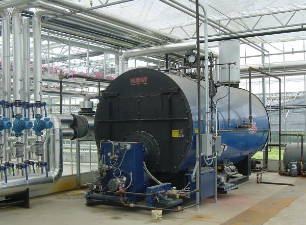
Hot Water Heating Systems

Water-based heating systems consist of a boiler and a water circulation system (pumps, mixing valves, and plumbing) (Figure 5.1.8). The boiler generates the heat to raise the temperature of the circulating water. The heated water is pumped to heat the greenhouse through a pipe network or tube distribution system. Usually, the heating pipes are installed on the support posts, around the perimeter, and overhead (sometimes near gutters to enhance snowmelt using the released heat, and spaced evenly between more widely spaced gutters to provide uniform heat delivery). Some greenhouses have floor or bench heating with additional heating tubes installed in the floor or on/near the benches for root-zone heating. These root-zone heating systems have the advantage of providing independent control of root-zone temperatures and delivering uniform heat very close to the plant canopy. However, root-zone heating systems are typically not able to provide sufficient heating capacity during the coldest times of the year, necessitating the use of additional heating in the form of perimeter and overhead heating pipes. A significant benefit of water-based heating systems is the ability to “store” heat in large insulated water tanks. Boilers can be used during the day to produce CO₂ for plant consumption, with any surplus heat stored for use during colder periods such as the night, when CO₂ supplementation is not required.

Figure \(\PageIndex{8}\): Hot water heating system including a boiler, mixing valves, pumps, and distribution plumbing (Photo by A. J. Both).

Infrared Heating Systems

Infrared heating systems have the advantage of immediate heat delivery once turned on, but only exposed (in terms of line-of-sight) plant canopy surfaces will receive the radiant heat. Infrared heating sometimes provides non-uniform heating, especially in crops with a multi-layered canopy. Also, infrared heating systems are typically designed as line sources and require some distance between the source and the radiated canopy surfaces to accomplish uniform distribution. Finally, like hot air systems, infrared heating systems accumulate little heat storage during operation, so that in case of an emergency shutdown, little residual heat is available to extend the heating time before the temperature drops below critical levels.

Alternative Energy Sources and Energy Conservation

The volatility in fossil fuel prices experienced during the last decades has put a greater emphasis on energy conservation and alternative energy sources. Energy conservation measures employed include relatively simple measures such as sealing unintended cracks and openings in the greenhouse glazing, improved insulation of structural components and heat transportation systems, and timely equipment maintenance, as well as more advanced measures such as movable insulation/shade curtains, new heating equipment with higher efficiencies (e.g., condensing boilers, heat pumps, combined heat and power systems), and novel control strategies (e.g., temperature integration, where growers are more concerned with the average temperature a crop receives, within set boundaries, rather than tightly maintaining a specific set point temperature). Some growers delay crop production to periods when the weather is warmer, while others use lower set point temperatures (often requiring more extended production periods and with potential impacts on plant physiology).

Alternative energy heating sources (i.e., non-fossil fuels) used for greenhouse applications include solar electric, solar thermal, wind, hydropower, biomass, and geothermal (co-generation and ground-source, shallow or deep). Many alternative energy installations are viable only under specific climatic conditions and may require significant investments that may require (local or national) financial incentives. Developing energy conservation and alternative energy strategies for greenhouse operations remains challenging because of the considerable differences in size, scope, and local circumstances. Selecting an alternative energy system includes considering economic viability for the greenhouse operation as well as protection of the environment.

Evaporative Cooling Systems

Growers or greenhouse managers often use evaporative cooling as the most affordable way of reducing the air temperature beyond what the ventilation system can achieve by air movement only. The maximum amount of cooling provided by evaporative cooling systems depends on the initial temperature and humidity of the ambient (i.e., outdoor) air. These parameters can be measured relatively easily with a standard thermometer and a relative humidity sensor. With these measurements, the psychrometric chart can be used to determine the corresponding properties of the air, such as the wet-bulb temperature, humidity ratio, enthalpy, etc. With the known wet-bulb temperature, the wet-bulb depression can be calculated to determine the theoretical temperature drop possible by evaporative cooling. Since few engineered systems are 100% efficient, the actual temperature drop achieved by the evaporative cooling system is likely to be 80–90% of the theoretical wet-bulb depression.

Lighting System Design

The concepts described earlier can be used to control the instantaneous intensity and integrated light intensities needed to assess the light conditions in plant growth facilities. The information can be used to determine the parameters needed to select fixtures to modify the light environment in plant growth facilities, e.g., switching the supplemental lighting system on or off, opening or closing a shade curtain (in greenhouses) and, when multi-spectral LEDs are used, can include changing the light spectrum and/or their overall intensity.

Light Requirements

In designing a lighting system for a greenhouse or indoor growing facility, the first step is to determine the light requirements of a particular crop. Research articles or grower handbooks for the crop of interest can provide information about the recommended light intensity and/or the optimum daily light integral (see, for example, Lopez and Runkle, 2017). For crops such as leafy greens grown in a greenhouse, the minimum daily target integral may be as low as 8 to 14 mol m⁻² d⁻¹, or as high as 17 mol m⁻² d⁻¹ (the maximum daily integral for leaf lettuce before physiological damage occurs as a result of too much light). For vine crops, such as tomatoes, a minimum of 15 mol m⁻² d⁻¹ is typically tolerated, while the optimum target can exceed 30 mol m⁻² d⁻¹. Generally, as a rule of thumb, for vegetable crops, a 1% increase in the DLI results in a 1% increase in growth (up to a point; Marcelis et al., 2006). Considering the high cost of providing the optimum growing environment, it usually makes economic sense to optimize plant growth whenever possible (Kubota et al., 2016).

Once the DLI for the crop has been determined, the next step is to determine how much supplemental lighting is required to make up any shortfall in natural light. In an indoor growing facility, all light must be supplied by electric lamps, while in a greenhouse, natural lighting typically provides the bulk of the DLI throughout the year. Even in relatively gloomy regions the sun can provide over 70% of the required light for a year-round greenhouse lettuce crop.

Supplemental lighting for greenhouse production is mostly used during the dark winter months when the sun is low and the days are short. Typically, greenhouse lighting systems are designed such that they can provide enough light during the darkest months of the year. To estimate the amount of light available for crop production at a particular location, ideally one would average several years of data so that an atypical year would have a minor impact on the overall trends. In the U.S., a useful resource is the National Solar Radiation Database maintained by the National Renewable Energy Laboratory (NREL) in Golden, Colorado (https://nsrdb.nrel.gov/).

The solar radiation data (i.e., shortwave radiation covering the waveband of approximately 300–3,000 nm) available from NREL is not specifically used for plant production and is usually expressed in units of J m⁻² per unit of time (e.g., an hour or a day). To convert this to a form more useful for planning supplemental lighting systems, the following multiplier can be used (Ting and Giacomelli, 1987):

\[ 1\frac{MJ}{m^{2}\text{day}}\text{short wave radiation}=2.0804\frac{\text{mol}}{m^{2}\text{day}}\text{PAR} \]

The NREL database covers several locations outside of the USA. For more specific location data, other weather databases maintained by national governments or local weather stations (e.g., radio or TV stations, airports) may have historic solar radiation data available from which average natural daily light integrals can be calculated.

For greenhouse production, the DLI does not have to be exactly the same each day to maximize production. During the seedling stage, many crops can tolerate DLIs much higher than during later stages of growth. For example, greenhouse lettuce typically is limited to 17 mol m⁻² d⁻¹ after the canopy has closed, to avoid damage from tipburn (Albright et al., 2000). However, seedlings can be provided with 20 mol m⁻² d⁻¹ and some varieties may even benefit from up to 30 mol m⁻² d⁻¹. Generally, for hydroponic lettuce, deviating no more than 3 mol m⁻² d⁻¹ from the target DLI is acceptable, provided any surplus (or deficit) is compensated for over the following two days.

Once the amount of supplemental lighting necessary has been determined (whether 100% of the DLI for an indoor growing facility or some other fraction of the DLI for a greenhouse), the next step is to determine what intensity of light is required. For indoor facilities, determining the required crop light level is straightforward. For a crop such as lettuce where there is no requirement for a night break, 24 hours of light per day can be applied. For a greenhouse, the calculation is the same, however, a portion of the DLI will be supplied by natural light. It comes down to a judgement call by the designer with respect to how they want to size the lighting system, and if they want to over- or under-size the lighting capacity to consider extremely dark days when the supplemental lighting system would need to provide nearly all of the light in a greenhouse. Most commercial greenhouse supplemental lighting systems provide an instantaneous intensity between 50 and 200 μmol m⁻² s⁻¹ at crop level.

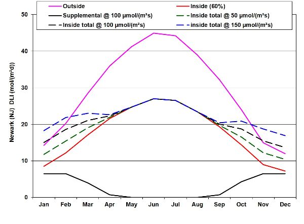
Figure 5.1.9 shows the increase in DLI that can be realized by adding supplemental lighting at three different intensities (50, 100, and 150 μmol m⁻² s⁻¹), while operating the lamps for 18 hours per day during November, December, January, and February, for 12 hours per day during October, for 11 hours per day during March, and 2 hours per day during September and April for a total of 2,993 hours per year. As shown in Figure 5.1.9, using this lighting schedule and an intensity of 150 μmol m⁻² s⁻¹ results in a more constant light integral over the course of a year.

Figure \(\PageIndex{9}\): Outside and inside solar radiation integrals (DLI, assuming 60% transmission and averaged by month) for Newark, NJ, USA. The dashed lines indicate the inside radiation integrals after operating a supplemental lighting system at three different light intensities (50, 100, and 150 μmol m⁻² s⁻¹) for different periods of time. See text for lighting system operating times.

A significant factor affecting the hours per day that supplemental lighting should be supplied is electricity pricing. Many utilities offer incentives to encourage off-peak usage of electricity, to even out the demand for electricity to all of their customers. It varies by utility providers, but savings as high as 40% on the supply charges of electricity are common for purchasing off-peak power. Typical off-peak periods correspond with nighttime and early morning, for example from 9:00 pm to 7:00 am (10 hours). In addition to saving on the supply price of electricity, it may be possible to avoid demand charges as well. In commercial operations that use a lot of power, electric utilities often collect demand charges based on the largest 15-minute on-peak consumption (kW) during a monthly billing cycle. The demand charge can easily add thousands of dollars to the monthly cost of a grower’s electricity bill. During winter months, it may be unavoidable to light during peak use hours, but during the shoulder months when supplemental lighting is still necessary but is not used as much, it may be worthwhile to disable lighting during on-peak hours and make up any daily deficit the next day during off-peak hours.

Number of Fixtures to Achieve a Target Intensity

The number of fixtures needed to provide the desired intensity depends on the light output of each fixture and the mounting height. In addition, the characteristics of any reflector will affect both the uniformity and intensity of light delivered to the crop (Ciolkosz et al., 2001; Both et al., 2002). The mounting height is defined as the distance between the bottom of the lamp and the top of the plant canopy.

Ideally, the lighting manufacturer will have available an IES (Illuminating Engineering Society) file that contains data on the specific light output pattern of the fixture. Using the IES file and commercially available software, it is possible to design a layout to achieve a target light intensity at a specified mounting height. An additional consideration is the uniformity of the light. Ideally, the light should be as uniform as possible to produce consistent growth throughout the growing area. Keep in mind that, although the light intensity does not change much once the lamp density is determined (Table 5.1.5), light uniformity significantly improves with increasing mounting height. For example, a 0.4 ha greenhouse (assuming an available mounting height of 2.44 m) would need approximately 383 HPS lamps (400 W each, not including the power drawn by the ballast) for a uniform light intensity of 49 μmol m⁻² s⁻¹ and 786 lamps for the intensity of 100 μmol m⁻² s⁻¹. Additional mounting patterns and resulting average light intensities are shown in Table 5.1.5.

Table \(\PageIndex{5}\): Estimated average light intensities at the top of the plant canopy (in μmol m⁻² s⁻¹) throughout a 0.4 ha greenhouse (10 gutter-connected bays of 7.3 m wide by 54.9 m long) for four different mounting heights and 400-watt HPS lamps. Note that these average light intensities are estimates without including edge effects (i.e., a drop in light intensity toward the outside walls) and these light intensities are estimates only; always consult with a trained lighting designer for an accurate calculation of expected light intensities in greenhouses.

Number of Lamps per Bay (lamps per row, with lamp placement staggered from row to row)	Floor Area per Lamp (m^2)	Light Intensity for a Mounting Height of 2.44 m (μmol m^−2 s^−1)	Light Intensity for a Mounting Height of 2.13 m (μmol m^−2 s^−1)	Light Intensity for a Mounting Height of 1.83 m (μmol m^−2 s^−1)	Light Intensity for a Mounting Height of 1.52 m (μmol m^−2 s^−1)
38 (13-12-13)	10.6	49	50	51	52
58 (15-14-15-14)	6.9	75	77	79	80
78 (16-15-16-15-16)	5.15	100	103	105	107
123 (21-20-21-20-21-20)	3.26	149	154	158	162
158 (23-22-23-22-23-22-23)	2.54	202	206	210	213

An additional consideration in greenhouses is that increasing the number of fixtures results in additional blockage of the natural light. Furthermore, power supply wires, ballasts, and reflectors can all block the transmission of natural light, and the greenhouse may require additional superstructure to provide a place to mount the fixtures and help support their weight.

Examples

Example \(\PageIndex{1}\)

Example 1: Greenhouse heating

Problem:

Determine the required heating system capacity for a greenhouse with the following characteristics:

• • greenhouse dimensions: 330 by 330 m
• • greenhouse surface area (roof plus sidewalls): 12,700 m²
• • greenhouse volume: 50,110 m³
• • outdoor humidity level: 45%
• • nighttime temperature set point: 17°C
• • indoor humidity level: 75%
• • 99% design temperature (location specific): −15°C
• • greenhouse U-value: 6.2 W m⁻² °C⁻¹

Solution

The required heating system capacity is a function of the structural heat loss (conduction, convection, and radiation), the infiltration heat loss, and the conversion efficiency of the fuel source for the heating system.

First, calculate the structural heat loss using Equation 5.1.1:

\( q_{ccr}=UA_{c}(t_{i}-t_{o}) \) (Equation \(\PageIndex{1}\))

= 6.2 × 12,700 [17 – (−15)] = 2,519,680 W = 2,519.68 kW

Next, determine the heat loss by infiltration using Equation 5.1.2:

\( q_{i}=\rho _{i}NV[c_{pi}(t_{i}-t_{o})+h_{fg}(W_{i}-W_{o})] \) (Equation \(\PageIndex{2}\))

Some assumptions are required to solve Equation 5.1.2. It is reasonable to assume that the air density of the greenhouse air is 1.2 kg m⁻³. The infiltration rate N can be estimated from data included in Table 5.1.2: a value of 0.0004 s⁻¹ was selected (an older, glass-covered greenhouse with good maintenance). In order to determine the humidity ratios for the inside and outside air, we need to use the relative humidity of the inside and outside air. Using the psychrometric chart (Figure 5.1.1), the humidity ratios for the inside and outside air are 0.0091 and 0.0005 kg kg⁻¹, respectively. The specific heat of greenhouse air at 17°C is 1.006 kJ kg ⁻¹ K⁻¹ and the latent heat of vaporization of water at that temperature is approximately 2,460 kJ kg⁻¹. These values were determined from online calculators (Engineering ToolBox, 2004, 2010), but can also commonly be found in engineering textbooks regarding heat and mass transfer. Entering these values in Equation 5.1.2:

\( q_{i}=\rho _{i}NV[c_{pi}(t_{i}-t_{o})+h_{fg}(W_{i}-W_{o})] \) (Equation \(\PageIndex{2}\))

= 1.2 × 0.0004 × 50,110 {1.006[17 – (−15)] + 2,460(0.0091–0.0005)}

= 1,283,169 W = 1,283.17 kW

Thus, the resulting heat loss is the sum of the structural heat loss (conduction, convection, and radiation) and the infiltration heat loss: 2,519.68 + 1,283.17 = approximately 3803 kW.

The heating system capacity is the total heat loss divided by the conversion efficiency of the fuel source. For natural gas with a conversion efficiency of 85%, the required overall heating system capacity is 3803/0.85 = 4,474 kW.

Note that if these calculations are done in a spreadsheet, it is easy to adjust the assumptions that were made so that the sensitivity of the final answer to the magnitude of the assumptions can be assessed. Also, in colder climates, additional heat can be lost around the perimeter of a greenhouse where cold and wet soil is in direct contact with the perimeter walkway inside the greenhouse. To prevent this perimeter heat loss, vertically placed insulation boards can be installed extending from ground level to a depth of 50–60 cm.

Example \(\PageIndex{2}\)

Example 2: Evaporative Cooling Pad

Problem:

Find the expected temperature drop of the air passing through the evaporative cooling pad given the following information:

• • the ambient (outside air) is at 25°C dry-bulb temperature and 50% relative humidity
• • the evaporative cooling pad efficiency is 80%

Solution

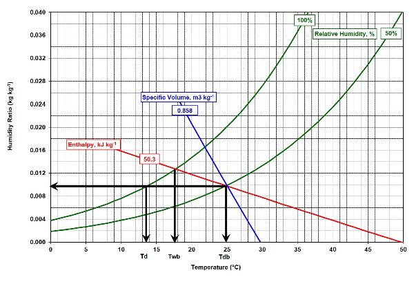
Using the psychrometric chart (Figure 5.1.10) and the initial conditions of the outside air of 25°C dry-bulb temperature and 50% relative humidity, start at the intersection of the curved 50% RH line with the vertical line for a dry-bulb temperature of 25°C. At this intersection, determine the following environmental parameters:

• • wet-bulb temperature = 17.8°C (from the starting point, follow the constant enthalpy line, 50.3 kJ kg⁻¹ in this case, until it intersects with the 100% relative humidity curve)
• • dew point temperature = 13.7°C
• • humidity ratio = 0.0099 kg kg⁻¹,
• • enthalpy = 50.3 kJ kg⁻¹
• • specific volume = 0.858 m³ kg⁻¹

Thus, the wet-bulb depression for this example equals 25 – 17.8 = 7.2°C. Using an overall evaporative cooling system efficiency of 80% results in a practical temperature drop of approximately 5.8°C (7.2°C × 0.8). As the air continues to travel through the greenhouse on its way to the exhaust fans, the exiting air will be warmed, and moisture from crop transpiration will be added so the exiting air will have higher energy content and specific humidity than the air moving through the evaporative cooling pad.

Figure \(\PageIndex{10}\): Simplified psychrometric chart used to visualize the evaporative cooling example described in the text. T_d = dew point temperature, T_wb = wet-bulb temperature, and T_db = dry-bulb temperature.

Example \(\PageIndex{3}\)

Example 3: Purchase and operating costs of crop lighting systems

Problem:

As mentioned previously, the performance of lamps in terms of their efficacy can vary significantly even when comparing the same type of lamp. For example, we measured HPS fixture efficacy values ranging from 0.94 to 1.7 μmol J⁻¹. Along with the efficacy, the unit cost of purchasing lamps is also an important consideration when deciding on a lighting system. In this example, we look at the cost of purchasing and operating two types of lighting systems, in both a greenhouse and an indoor growing facility.

Find the yearly cost savings of operating an LED vs. HPS system, and how long the systems should be operated to justify (payback) the higher purchase price of the LED lighting system, in both a greenhouse and indoor (no natural light) production system, given the following:

• • HPS lighting system: 123 fixtures, each 400 W (plus 60 W for each ballast), cost of $300 per fixture (excluding installation cost), efficacy of 0.94 μmol J⁻¹
• • LED lighting system: 55 fixtures, each 400 W (plus 20 W for each driver), cost of $1,200 per fixture (excluding installation cost), efficacy of 2.1 μmol J⁻¹ (these LED fixtures are intended as a direct replacement for the HPS lighting system, meaning they deliver the same PAR intensity and distribution at crop level)
• • Greenhouse: 2,200 hours of supplemental lighting per year (600 h during on-peak electricity rates and 1,600h during off-peak electricity rates)
• • Indoor (no natural light) growing facility: 8,760 hours of lighting per year (5,100 h on-peak and 3,660 h off-peak)
• • Electricity prices of $0.14 per kWh on-peak, and $0.09 per kWh off-peak.

Solution

We can now compare the cost to purchase and operate the fixtures. The purchase price of the two systems is simply the unit cost multiplied by the number of units:

\( \text{HPS purchase cost}=\frac{\$ 300}{\text{fixture}}\times 123 \text{ fixtures} = \$ 36,900 \)

\( \text{LED purchase cost}=\frac{\$ 1,200}{\text{fixture}}\times 55 \text{ fixtures} = \$ 66,000 \)

For the greenhouse case, the electricity cost of the two lighting systems can be determined for both on-peak and off-peak use:

\( \text{HPS on-peak cost}= 123 \text{ fixtures} \times \frac{460\ W}{\text{fixture}}\times \frac{1\ kW}{1000\ W}\times \frac{600 \text{ h on-peak}}{\text{year}} \times \frac{\$ 0.14}{kWh} =\frac{\$ 4,753}{\text{year}} \)

\( \text{HPS off-peak cost}= 123 \text{ fixtures} \times \frac{460\ W}{\text{fixture}}\times \frac{1\ kW}{1000\ W}\times \frac{1,600 \text{ h off-peak}}{\text{year}} \times \frac{\$ 0.09}{kWh} =\frac{\$ 8,148}{\text{year}} \)

Adding these costs results in an annual electricity cost for HPS of $12,901 per year (excluding any potential demand charges).

\( \text{LED on-peak cost}= 55 \text{ fixtures} \times \frac{420\ W}{\text{fixture}}\times \frac{1\ kW}{1000\ W}\times \frac{600 \text{ h on-peak}}{\text{year}} \times \frac{\$ 0.14}{kWh} =\frac{\$ 1,940}{\text{year}} \)

\( \text{LED off-peak cost}= 55 \text{ fixtures} \times \frac{420\ W}{\text{fixture}}\times \frac{1\ kW}{1000\ W}\times \frac{1,600 \text{ h on-peak}}{\text{year}} \times \frac{\$ 0.09}{kWh} =\frac{\$ 3,326}{\text{year}} \)

Adding these costs results in an annual electricity cost for LED of $5,266 per year (excluding any potential demand charges).

The annual cost savings for electricity consumption by using the LED instead of the HPS fixtures amounts to $12,901 – $5,266 = $7,635.

The premium for purchasing LED instead of the HPS fixtures is $29,100 ($66,000 – $36,900). Therefore, it would take \(\frac{\$ 29,100}{\$ 7,635} = 3.8\text{ years}\) of operation to recover (pay back) the higher purchase price of the LED fixtures in the greenhouse situation.

For the case of an indoor growing facility, where all of the lighting had to be supplied by the lamp fixtures, and assuming the lights needed to operate 24 hours a day to meet the target light integral, the annual cost savings for electricity consumption by using the LED instead of the HPS fixtures amounts to $34,933 ($50,035 – $24,102). Therefore, it would take \(\frac{\$ 29,100}{\$ 34,933} = 0.83\text{ years}\) of operation to recover (pay back) the higher purchase price of the LED fixtures.

Image Credits

Figure 1. Both, A. J. (CC By 4.0). (2020). Psychrometric chart.

Figure 2. Both, A. J. (CC By 4.0). (2020). Evaporative cooling system (pad and fan).

Figure 3. Both, A. J. (CC By 4.0). (2020). Gutter-connected greenhouses.

Figure 4. Both, A. J. (CC By 4.0). (2020). Sensitivity of human eye and plant.

Figure 5. Left. Both, A. J. (2020). Lettuce plants.

Figure 5. Right. Cornell University. (CC By 4.0). Lettuce Plants. Retrieved from https://urbanagnews.com/blog/prevent-tipburn-on-greenhouse-lettuce/. [Fair Use].

Figure 6. Both, A. J. (CC By 4.0). (2020). HPS and LED fixtures.

Figure 7. Both, A. J. (CC By 4.0). (2020). Unit heater.

Figure 8. Both, A. J. (CC By 4.0). (2020). Hot water heating system.

Figure 9. Both, A. J. (CC By 4.0). (2020). Solar radiation integrals.

Figure 10. Both, A. J. (CC By 4.0). (2020). Simplified psychrometric chart.

References

Albright, L. D., Both, A. J., & Chiu, A. J. (2000). Controlling greenhouse light to a consistent daily integral. Trans. ASAE, 43(2), 421–431. https://doi.org/10.13031/2013.2721.

Aldrich, R. A., & Bartok, J. W. (1994). Greenhouse engineering. NRAES Publ. No. 33. Retrieved from https://vdocuments.site/fair-use-of-this-pdf-file-of-greenhouse-engineering-nraes-33-by-.html.

ASABE Standards. (2017). ANSI/ASABE S640: Quantities and units of electromagnetic radiation for plants (photosynthetic organisms). St. Joseph, MI: ASABE.

ASAE Standards. (2003). ANSI/ASAE EP406.4: Heating, ventilating, and cooling greenhouses. Note: This is a withdrawn and archived standard. St. Joseph, MI: ASAE.

ASHRAE. (2013). ASHRAE Standard 169-2013: Weather data for building design standards. Atlanta, GA: ASHRAE.

Both, A. J., Albright, L. D., Langhans, R. W., Vinzant, B. G., & Walker, P. N. (1997). Electric energy consumption and PPF output of nine 400 Watt high pressure sodium luminaires and a greenhouse application of the results. Acta Hortic., 418, 195–202.

Both, A. J., Benjamin, L., Franklin, J., Holroyd, G., Incoll, L. D., Lefsrud, M. G., & Pitkin, G. (2015). Guidelines for measuring and reporting environmental parameters for experiments in greenhouses. Plant Methods, 11(43). https://doi.org/10.1186/s13007-015-0083-5.

Both, A. J., Bugbee, B., Kubota, C., Lopez, R. G., Mitchell, C., Runkle, E. S., & Wallace, C. (2017). Proposed product label for electric lamps used in the plant sciences. HortTechnol., 27(4), 544–549. https://doi.org/10.21273/horttech03648-16.

Both, A. J., Ciolkosz, D. E., & Albright, L. D. (2002). Evaluation of light uniformity underneath supplemental lighting systems. Acta Hortic., 580, 183–190.

Ciolkosz, D. E., Both, A. J., & Albright, L. D. (2001). Selection and placement of greenhouse luminaires for uniformity. Appl. Eng. Agric., 17(6), 875–882. https://doi.org/10.13031/2013.6842.

Commission Internationale de l’Eclairage. (1931). Proc. Eighth Session. Cambridge, UK: Cambridge University Press.

Crawley, D. B., Lawrie, L. K., Winkelmann, F. C., Buhl, W. F., Huang, Y. J., Pedersen, C.O., . . . Glazer, J. (2001). EnergyPlus: Creating a new-generation building energy simulation program. Energy Build., 33(4), 319–331. http://dx.doi.org/10.1016/S0378-7788(00)00114-6.

Engineering ToolBox. (2004). Air—Specific heat at constant pressure and varying temperature. Retrieved from https://www.engineeringtoolbox.com/air-specific-heat-capacity-d_705.html.

Engineering ToolBox. (2010). Water—Heat of vaporization. Retrieved from https://www.engineeringtoolbox.com/water-properties-d_1573.html.

Kubota, C., Kroggel, M., Both, A. J., Burr, J. F., & Whalen, M. (2016). Does supplemental lighting make sense for my crop?—Empirical evaluations. Acta Hortic., 1134, 403–411. http://dx.doi.org/10.17660/ActaHortic.2016.1134.52.

Lopez, R., & Runkle, E. S. (Eds.). (2017). Light management in controlled environments. Willoughby, OH: Meister Media Worldwide.

Marcelis, L. F. M., Broekhuijsen, A. G. M., Meinen, E., Nijs, E. M. F. M., & Raaphorst, M. G. M. (2006). Quantification of the growth response to light quantity of greenhouse grown crops. Acta Hortic., 711, 97–103. https://doi.org/10.17660/ActaHortic.2006.711.9.

Mitchell, C. A., Both, A. J., Bourget, C. M., Burr, J. F., Kubota, C., Lopez, R. G., . . . Runkle, E. S. (2012). LEDs: The future of greenhouse lighting! Chron. Hortic., 52(1), 6–12.

Mitchell, C. A., Dzakovich, M. P., Gomez, C., Lopez, R., Burr, J. F., Hernandez, R., . . . Both, A. J. (2015). Light-emitting diodes in horticulture. Hortic. Rev., 43, 1–87.

Sager, J. C., Smith, W. O., Edwards, J. L., & Cyr, K. L. (1988). Photosynthetic efficiency and phytochrome photoequilibria determination using spectral data. Trans. ASAE, 31(6), 1882–1889. https://doi.org/10.13031/2013.30952.

Ting, K. C., & Giacomelli, G. A. (1987). Availability of solar photosynthetically active radiation. Trans. ASAE, 30(5), 1453–1457. https://doi.org/10.13031/2013.30585.

USDA-ARS. (2019). Virtual grower 3.0. Washington, DC: U.S. Department of Agriculture. https://www.ars.usda.gov/research/software/download/?softwareid=309.

Wallace, C. & Both, A. J. (2016). Evaluating operating characteristics of light sources for horticultural applications. Acta Hortic., 1134, 435–443. https://doi.org/10.17660/ActaHortic.2016.1134.55.